MS Excel VLookup issue

Question

Good day!

MS Excel VLOOKUP issue;

• i'm getting #N/A result
• it should be YES because im vlookup is looking for Item No_?
• im missing something in my formula

Thank you.

Table:

VLOOKUP result;

Answer 1

In your first formula you have the range starting at A5 and the second starts at A2. It looks as though A5 in your range doesn't equal 1001498.

Answer 2

I know you may have had your question answered. If someone else sees this question and it doesn't answer theirs, they can try this one too.

If your vlookup is correct and includes the dollar signs, it might be a cell-format issue. To fix the cell format, you might try this:

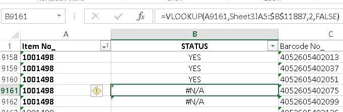
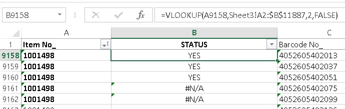
=VLOOKUP(A9158*1,Sheet3!A2:$B$11887,2,FALSE)  

Adding "*1" will convert the text to a number and will then look up the value as a number.

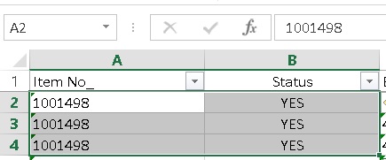
Sometimes, a number is in a cell stored as text or vice-versa (the text is stored as a number if it only has numbers in it). Because you have left-aligned your column values, you might not be able to tell easily.

A Few Different Approaches (use what's easiest for you)
To format all of your values as text, select all of the values in the column, then go to Home>Number and select "Text" from the dropdown menu (don't select "General"). Even though your numbers/values look left aligned, don't let it fool you - they're still in number format. To get the values into text format, try one of these several approaches:

1. add ' to the beginning of your number. For example '200023134 instead of 200023134. Formulas will ignore the ', and will still recognize the number as a text value.
2. After changing the cell format to text, double-click inside the cell. It will convert the number to a text value that still looks like the number.
3. If you have too many values to try the above two methods, try one of these: 3a. insert a new blank column, and add the following formula: =TEXT(A9158 (or whatever cell has the value in it that you want to change to text), "0"). Drag the formula down, and then copy/paste-as-values the results into the column containing your original numbers. 3b. Open Notepad. After changing the cell format to text, highlight your column of number values, copy/paste to Notepad, and then paste the values back into Excel. 3c. Select the range of values you want to convert to text, then go to Data>Text to columns. Select "Delimited" and Next>. Make sure all delimiters are unchecked and Next>. Select "Text" and Finish.

Additional Help
It's also good to do the same thing to the values you're trying to =VLOOKUP(this number, and this range), 2, FALSE). If you want the values all formatted as numbers, you can do the same thing, but format all as numbers. Otherwise, you may end up with some values not being found that actually exist - especially on longer lists of numbers or text.

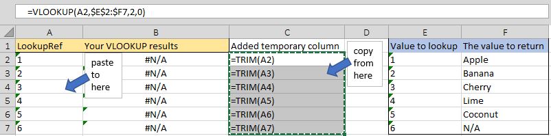
One other good tool is the =TRIM(cell reference). Sometimes, even though a cell value is formatted as text and your lookup value is also formatted as text, one value or the other may have invisible spaces at the end like this: "00100234023 " while the other value you're comparing it to might look like this: "00100234023". To do the TRIM formula, do this:

1. Create a new column next to the column of values you want to trim extra spaces from.
2. Type =TRIM("click on the adjacent cell you want to trim and don't add these quotes")
3. Copy the cells containing the formulas and paste them over the column containing your untrimmed values.

Visual example of The TRIM formula: