How to create pivot table with multiple headers in power query

Question

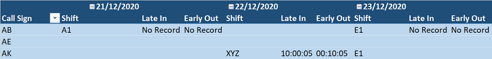
Hi, I have a problem to create pivot table with multiple headers in power query, here is my base data: ![73603-base-data.jpg][1] And, here is my expected output: ![73604-expected-output.jpg][2] How can i generate the expected output? Thanks a lot! [1]: /api/attachments/73603-base-data.jpg?platform=QnA [2]: /api/attachments/73604-expected-output.jpg?platform=QnA

Answer 1

Hi @Cherry

(next time please upload & share a workbook - i.e. with OneDrive - as creating dummy data takes time. Thanks)

The below solution involves Power Pivot in addition to Power Query. Assuming Excel SourceTable

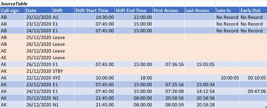
NOTE: It seems you're not interested by the orange rows (no [Shift Start Time]). If I misunderstood this, adjust line #10 (step FilteredOutNullShiftStart) in the below Power Query code:
EDIT: I forgot a point > If you always have at least 1 record where fields [Shift], [Late In] & [Early Out] are not null then steps ReplacedNulls and RestoredNulls are not required

// SourceTable  
let  
    Source = Excel.CurrentWorkbook(){[Name="SourceTable"]}[Content],  
    RequiredColumns = Table.SelectColumns(Source,  
        {"Call-sign", "Date", "Shift", "Shift Start Time", "Late In", "Early Out"}  
    ),  
    ChangedTypes = Table.TransformColumnTypes(RequiredColumns,  
        {<!-- -->{"Call-sign", type text}, {"Shift", type text}, {"Date", type date}}  
    ),  
    FilteredOutNullShiftStart = Table.SelectRows(ChangedTypes, each  
        ([Shift Start Time] <> null)  
    ),  
    RemovedShiftStartTime = Table.RemoveColumns(FilteredOutNullShiftStart,{"Shift Start Time"}),  
    ReplacedNulls = Table.ReplaceValue(RemovedShiftStartTime, null, "_Fake_Value_",  
        Replacer.ReplaceValue,{"Late In", "Early Out"}  
    ),  
    UnpivotedColumns = Table.UnpivotOtherColumns(ReplacedNulls,  
        {"Call-sign", "Date"}, "ColumnName", "Value"  
    ),  
    RestoredNulls = Table.ReplaceValue(UnpivotedColumns, "_Fake_Value_", null,  
        Replacer.ReplaceValue,{"Value"}  
    ),  
    TimeValueToText = Table.AddColumn(RestoredNulls, "TextValue", each  
        try Time.ToText(Time.From([Value]),"hh:mm:ss") otherwise [Value],  
        type text  
    ),  
    RemovedValue = Table.RemoveColumns(TimeValueToText,{"Value"})  
in  
    RemovedValue  

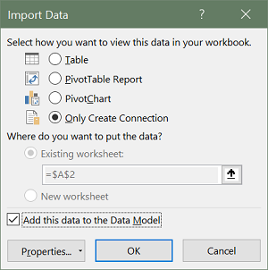
Load this query as a Connection Only + Add this data to the Data Model:

Within Excel go to the Power Pivot tab > Measures > New Measure... and create measure ValueToReport with DAX formula:

   =CONCATENATEX(SourceTable,SourceTable[TextValue],", ")  

Then create a Pivot Table from the Data Model with
[Call-sign] to Rows
[Date] & [ColumnName] to Columns
fxValueToReport to Values

Manually sort [ColumnName] (Shift, Late In, Early Out)
Remove Grand Total for Rows & Columns

Corresponding sample workbook avail. here

Answer 2

Thanks for your suggestion, however, our office is using standard version of Excel, cannot support Power pivot.

Any other suggestion for me? Thanks.

Answer 3

We are using standard 2013.

Answer 4

I need to process around 2500 records.