Data science with an Ubuntu Data Science Virtual Machine in Azure
This walkthrough shows you how to complete several common data science tasks by using the Ubuntu Data Science Virtual Machine (DSVM). The Ubuntu DSVM is a virtual machine image available in Azure that's preinstalled with a collection of tools commonly used for data analytics and machine learning. The key software components are itemized in Provision the Ubuntu Data Science Virtual Machine. The DSVM image makes it easy to get started doing data science in minutes, without having to install and configure each of the tools individually. You can easily scale up the DSVM if you need to, and you can stop it when it's not in use. The DSVM resource is both elastic and cost-efficient.
In this walkthrough, we analyze the spambase dataset. Spambase is a set of emails that are marked either spam or ham (not spam). Spambase also contains some statistics about the content of the emails. We talk about the statistics later in the walkthrough.
Prerequisites
Before you can use a Linux DSVM, you must have the following prerequisites:
Azure subscription. To get an Azure subscription, see Create your free Azure account today.
Ubuntu Data Science Virtual Machine. For information about provisioning the virtual machine, see Provision the Ubuntu Data Science Virtual Machine.
X2Go installed on your computer with an open XFCE session. For more information, see Install and configure the X2Go client.
Download the spambase dataset
The spambase dataset is a relatively small set of data that contains 4,601 examples. The dataset is a convenient size for demonstrating some of the key features of the DSVM because it keeps the resource requirements modest.
Note
This walkthrough was created by using a D2 v2-size Linux DSVM. You can use a DSVM this size to complete the procedures that are demonstrated in this walkthrough.
If you need more storage space, you can create additional disks and attach them to your DSVM. The disks use persistent Azure storage, so their data is preserved even if the server is reprovisioned due to resizing or is shut down. To add a disk and attach it to your DSVM, complete the steps in Add a disk to a Linux VM. The steps for adding a disk use the Azure CLI, which is already installed on the DSVM. You can complete the steps entirely from the DSVM itself. Another option to increase storage is to use Azure Files.
To download the data, open a terminal window, and then run this command:
wget --no-check-certificate https://archive.ics.uci.edu/ml/machine-learning-databases/spambase/spambase.data
The downloaded file doesn't have a header row. Let's create another file that does have a header. Run this command to create a file with the appropriate headers:
echo 'word_freq_make, word_freq_address, word_freq_all, word_freq_3d,word_freq_our, word_freq_over, word_freq_remove, word_freq_internet,word_freq_order, word_freq_mail, word_freq_receive, word_freq_will,word_freq_people, word_freq_report, word_freq_addresses, word_freq_free,word_freq_business, word_freq_email, word_freq_you, word_freq_credit,word_freq_your, word_freq_font, word_freq_000, word_freq_money,word_freq_hp, word_freq_hpl, word_freq_george, word_freq_650, word_freq_lab,word_freq_labs, word_freq_telnet, word_freq_857, word_freq_data,word_freq_415, word_freq_85, word_freq_technology, word_freq_1999,word_freq_parts, word_freq_pm, word_freq_direct, word_freq_cs, word_freq_meeting,word_freq_original, word_freq_project, word_freq_re, word_freq_edu,word_freq_table, word_freq_conference, char_freq_semicolon, char_freq_leftParen,char_freq_leftBracket, char_freq_exclamation, char_freq_dollar, char_freq_pound, capital_run_length_average,capital_run_length_longest, capital_run_length_total, spam' > headers
Then, concatenate the two files together:
cat spambase.data >> headers
mv headers spambaseHeaders.data
The dataset has several types of statistics for each email:
- Columns like word_freq_WORD indicate the percentage of words in the email that match WORD. For example, if word_freq_make is 1, then 1% of all words in the email were make.
- Columns like char_freq_CHAR indicate the percentage of all characters in the email that are CHAR.
- capital_run_length_longest is the longest length of a sequence of capital letters.
- capital_run_length_average is the average length of all sequences of capital letters.
- capital_run_length_total is the total length of all sequences of capital letters.
- spam indicates whether the email was considered spam or not (1 = spam, 0 = not spam).
Explore the dataset by using R Open
Let's examine the data and do some basic machine learning by using R. The DSVM comes with CRAN R pre-installed.
To get copies of the code samples that are used in this walkthrough, use git to clone the Azure-Machine-Learning-Data-Science repository. Git is preinstalled on the DSVM. At the git command line, run:
git clone https://github.com/Azure/Azure-MachineLearning-DataScience.git
Open a terminal window and start a new R session in the R interactive console. To import the data and set up the environment:
data <- read.csv("spambaseHeaders.data")
set.seed(123)
To see summary statistics about each column:
summary(data)
For a different view of the data:
str(data)
This view shows you the type of each variable and the first few values in the dataset.
The spam column was read as an integer, but it's actually a categorical variable (or factor). To set its type:
data$spam <- as.factor(data$spam)
To do some exploratory analysis, use the ggplot2 package, a popular graphing library for R that's preinstalled on the DSVM. Based on the summary data displayed earlier, we have summary statistics on the frequency of the exclamation mark character. Let's plot those frequencies here by running the following commands:
library(ggplot2)
ggplot(data) + geom_histogram(aes(x=char_freq_exclamation), binwidth=0.25)
Because the zero bar is skewing the plot, let's eliminate it:
email_with_exclamation = data[data$char_freq_exclamation > 0, ]
ggplot(email_with_exclamation) + geom_histogram(aes(x=char_freq_exclamation), binwidth=0.25)
There is a nontrivial density above 1 that looks interesting. Let's look at only that data:
ggplot(data[data$char_freq_exclamation > 1, ]) + geom_histogram(aes(x=char_freq_exclamation), binwidth=0.25)
Then, split it by spam versus ham:
ggplot(data[data$char_freq_exclamation > 1, ], aes(x=char_freq_exclamation)) +
geom_density(lty=3) +
geom_density(aes(fill=spam, colour=spam), alpha=0.55) +
xlab("spam") +
ggtitle("Distribution of spam \nby frequency of !") +
labs(fill="spam", y="Density")
These examples should help you make similar plots and explore data in the other columns.
Train and test a machine learning model
Let's train a couple of machine learning models to classify the emails in the dataset as containing either spam or ham. In this section, we train a decision tree model and a random forest model. Then, we test the accuracy of the predictions.
Note
The rpart (Recursive Partitioning and Regression Trees) package used in the following code is already installed on the DSVM.
First, let's split the dataset into training sets and test sets:
rnd <- runif(dim(data)[1])
trainSet = subset(data, rnd <= 0.7)
testSet = subset(data, rnd > 0.7)
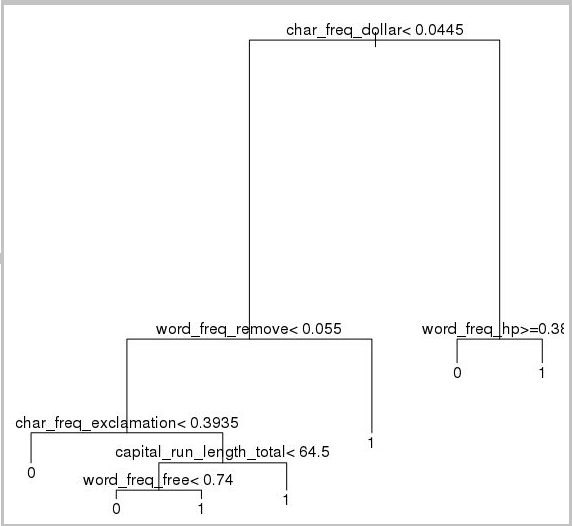
Then, create a decision tree to classify the emails:
require(rpart)
model.rpart <- rpart(spam ~ ., method = "class", data = trainSet)
plot(model.rpart)
text(model.rpart)
Here's the result:
To determine how well it performs on the training set, use the following code:
trainSetPred <- predict(model.rpart, newdata = trainSet, type = "class")
t <- table(`Actual Class` = trainSet$spam, `Predicted Class` = trainSetPred)
accuracy <- sum(diag(t))/sum(t)
accuracy
To determine how well it performs on the test set:
testSetPred <- predict(model.rpart, newdata = testSet, type = "class")
t <- table(`Actual Class` = testSet$spam, `Predicted Class` = testSetPred)
accuracy <- sum(diag(t))/sum(t)
accuracy
Let's also try a random forest model. Random forests train a multitude of decision trees and output a class that's the mode of the classifications from all the individual decision trees. They provide a more powerful machine learning approach because they correct for the tendency of a decision tree model to overfit a training dataset.
require(randomForest)
trainVars <- setdiff(colnames(data), 'spam')
model.rf <- randomForest(x=trainSet[, trainVars], y=trainSet$spam)

trainSetPred <- predict(model.rf, newdata = trainSet[, trainVars], type = "class")
table(`Actual Class` = trainSet$spam, `Predicted Class` = trainSetPred)

testSetPred <- predict(model.rf, newdata = testSet[, trainVars], type = "class")
t <- table(`Actual Class` = testSet$spam, `Predicted Class` = testSetPred)
accuracy <- sum(diag(t))/sum(t)
accuracy
Deep learning tutorials and walkthroughs
In addition to the framework-based samples, a set of comprehensive walkthroughs is also provided. These walkthroughs help you jump-start your development of deep learning applications in domains like image and text/language understanding.
Running neural networks across different frameworks: A comprehensive walkthrough that shows you how to migrate code from one framework to another. It also demonstrates how to compare model and runtime performance across frameworks.
A how-to guide for building an end-to-end solution to detect products within images: Image detection is a technique that can locate and classify objects within images. The technology has the potential to bring huge rewards in many real-life business domains. For example, retailers can use this technique to determine which product a customer has picked up from the shelf. This information in turn helps stores manage product inventory.
Deep learning for audio: This tutorial shows how to train a deep learning model for audio event detection on the urban sounds dataset. The tutorial provides an overview of how to work with audio data.
Classification of text documents: This walkthrough demonstrates how to build and train two different neural network architectures: Hierarchical Attention Network and Long Short Term Memory (LSTM). These neural networks use the Keras API for deep learning to classify text documents. Keras is a front end to three of the most popular deep learning frameworks: Microsoft Cognitive Toolkit, TensorFlow, and Theano.
Other tools
The remaining sections show you how to use some of the tools that are installed on the Linux DSVM. We discuss these tools:
- XGBoost
- Python
- JupyterHub
- Rattle
- PostgreSQL and SQuirreL SQL
- Azure Synapse Analytics (formerly SQL DW)
XGBoost
XGBoost provides a fast and accurate boosted tree implementation.
require(xgboost)
data <- read.csv("spambaseHeaders.data")
set.seed(123)

rnd <- runif(dim(data)[1])
trainSet = subset(data, rnd <= 0.7)
testSet = subset(data, rnd > 0.7)

bst <- xgboost(data = data.matrix(trainSet[,0:57]), label = trainSet$spam, nthread = 2, nrounds = 2, objective = "binary:logistic")

pred <- predict(bst, data.matrix(testSet[, 0:57]))
accuracy <- 1.0 - mean(as.numeric(pred > 0.5) != testSet$spam)
print(paste("test accuracy = ", accuracy))
XGBoost also can call from Python or a command line.
Python
For Python development, the Anaconda Python distributions 3.5 and 2.7 are installed on the DSVM.
Note
The Anaconda distribution includes Conda. You can use Conda to create custom Python environments that have different versions or packages installed in them.
Let's read in some of the spambase dataset and classify the emails with support vector machines in Scikit-learn:
import pandas
from sklearn import svm
data = pandas.read_csv("spambaseHeaders.data", sep = ',\s*')
X = data.ix[:, 0:57]
y = data.ix[:, 57]
clf = svm.SVC()
clf.fit(X, y)
To make predictions:
clf.predict(X.ix[0:20, :])
To demonstrate how to publish an Azure Machine Learning endpoint, let's make a more basic model. We'll use the three variables that we used when we published the R model earlier:
X = data[["char_freq_dollar", "word_freq_remove", "word_freq_hp"]]
y = data.ix[:, 57]
clf = svm.SVC()
clf.fit(X, y)
JupyterHub
The Anaconda distribution in the DSVM comes with a Jupyter Notebook, a cross-platform environment for sharing Python, R, or Julia code and analysis. The Jupyter Notebook is accessed through JupyterHub. You sign in by using your local Linux user name and password at https://<DSVM DNS name or IP address>:8000/. All configuration files for JupyterHub are found in /etc/jupyterhub.
Note
To use the Python Package Manager (via the pip command) from a Jupyter Notebook in the current kernel, use this command in the code cell:
 import sys
 ! {sys.executable} -m pip install numpy -y
To use the Conda installer (via the conda command) from a Jupyter Notebook in the current kernel, use this command in a code cell:
 import sys
 ! {sys.prefix}/bin/conda install --yes --prefix {sys.prefix} numpy
Several sample notebooks are already installed on the DSVM:
- Sample Python notebooks:
- Sample R notebook:
Note
The Julia language also is available from the command line on the Linux DSVM.
Rattle
Rattle (R Analytical Tool To Learn Easily) is a graphical R tool for data mining. Rattle has an intuitive interface that makes it easy to load, explore, and transform data, and to build and evaluate models. Rattle: A Data Mining GUI for R provides a walkthrough that demonstrates Rattle's features.
Install and start Rattle by running these commands:
if(!require("rattle")) install.packages("rattle")
require(rattle)
rattle()
Note
You don't need to install Rattle on the DSVM. However, you might be prompted to install additional packages when Rattle opens.
Rattle uses a tab-based interface. Most of the tabs correspond to steps in the Team Data Science Process, like loading data or exploring data. The data science process flows from left to right through the tabs. The last tab contains a log of the R commands that were run by Rattle.
To load and configure the dataset:
- To load the file, select the Data tab.
- Choose the selector next to Filename, and then select spambaseHeaders.data.
- To load the file. select Execute. You should see a summary of each column, including its identified data type; whether it's an input, a target, or other type of variable; and the number of unique values.
- Rattle has correctly identified the spam column as the target. Select the spam column, and then set the Target Data Type to Categoric.
To explore the data:
- Select the Explore tab.
- To see information about the variable types and some summary statistics, select Summary > Execute.
- To view other types of statistics about each variable, select other options, like Describe or Basics.
You can also use the Explore tab to generate insightful plots. To plot a histogram of the data:
- Select Distributions.
- For word_freq_remove and word_freq_you, select Histogram.
- Select Execute. You should see both density plots in a single graph window, where it's clear that the word you appears much more frequently in emails than remove.
The Correlation plots also are interesting. To create a plot:
- For Type, select Correlation.
- Select Execute.
- Rattle warns you that it recommends a maximum of 40 variables. Select Yes to view the plot.
There are some interesting correlations that come up: technology is strongly correlated to HP and labs, for example. It's also strongly correlated to 650 because the area code of the dataset donors is 650.
The numeric values for the correlations between words are available in the Explore window. It's interesting to note, for example, that technology is negatively correlated with your and money.
Rattle can transform the dataset to handle some common issues. For example, it can rescale features, impute missing values, handle outliers, and remove variables or observations that have missing data. Rattle can also identify association rules between observations and variables. These tabs aren't covered in this introductory walkthrough.
Rattle also can run cluster analysis. Let's exclude some features to make the output easier to read. On the Data tab, select Ignore next to each of the variables except these 10 items:
- word_freq_hp
- word_freq_technology
- word_freq_george
- word_freq_remove
- word_freq_your
- word_freq_dollar
- word_freq_money
- capital_run_length_longest
- word_freq_business
- spam
Return to the Cluster tab. Select KMeans, and then set Number of clusters to 4. Select Execute. The results are displayed in the output window. One cluster has high frequency of george and hp, and is probably a legitimate business email.
To build a basic decision tree machine learning model:
- Select the Model tab,
- For the Type, select Tree.
- Select Execute to display the tree in text form in the output window.
- Select the Draw button to view a graphical version. The decision tree looks similar to the tree we obtained earlier by using rpart.
A helpful feature of Rattle is its ability to run several machine learning methods and quickly evaluate them. Here's are the steps:
- For Type, select All.
- Select Execute.
- When Rattle finishes running, you can select any Type value, like SVM, and view the results.
- You also can compare the performance of the models on the validation set by using the Evaluate tab. For example, the Error Matrix selection shows you the confusion matrix, overall error, and averaged class error for each model on the validation set. You also can plot ROC curves, run sensitivity analysis, and do other types of model evaluations.
When you're finished building models, select the Log tab to view the R code that was run by Rattle during your session. You can select the Export button to save it.
Note
The current release of Rattle contains a bug. To modify the script or to use it to repeat your steps later, you must insert a # character in front of Export this log ... in the text of the log.
PostgreSQL and SQuirreL SQL
The DSVM comes with PostgreSQL installed. PostgreSQL is a sophisticated, open-source relational database. This section shows you how to load the spambase dataset into PostgreSQL and then query it.
Before you can load the data, you must allow password authentication from the localhost. At a command prompt, run:
sudo gedit /var/lib/pgsql/data/pg_hba.conf
Near the bottom of the config file are several lines that detail the allowed connections:
# "local" is only for Unix domain socket connections:
local   all             all                                     trust
# IPv4 local connections:
host    all             all             127.0.0.1/32            ident
# IPv6 local connections:
host    all             all             ::1/128                 ident
Change the IPv4 local connections line to use md5 instead of ident, so we can log in by using a username and password:
# IPv4 local connections:
host    all             all             127.0.0.1/32            md5
Then, restart the PostgreSQL service:
sudo systemctl restart postgresql
To launch psql (an interactive terminal for PostgreSQL) as the built-in postgres user, run this command:
sudo -u postgres psql
Create a new user account by using the username of the Linux account you used to log in. Create a password:
CREATE USER <username> WITH CREATEDB;
CREATE DATABASE <username>;
ALTER USER <username> password '<password>';
\quit
Log in to psql:
psql
Import the data to a new database:
CREATE DATABASE spam;
\c spam
CREATE TABLE data (word_freq_make real, word_freq_address real, word_freq_all real, word_freq_3d real,word_freq_our real, word_freq_over real, word_freq_remove real, word_freq_internet real,word_freq_order real, word_freq_mail real, word_freq_receive real, word_freq_will real,word_freq_people real, word_freq_report real, word_freq_addresses real, word_freq_free real,word_freq_business real, word_freq_email real, word_freq_you real, word_freq_credit real,word_freq_your real, word_freq_font real, word_freq_000 real, word_freq_money real,word_freq_hp real, word_freq_hpl real, word_freq_george real, word_freq_650 real, word_freq_lab real,word_freq_labs real, word_freq_telnet real, word_freq_857 real, word_freq_data real,word_freq_415 real, word_freq_85 real, word_freq_technology real, word_freq_1999 real,word_freq_parts real, word_freq_pm real, word_freq_direct real, word_freq_cs real, word_freq_meeting real,word_freq_original real, word_freq_project real, word_freq_re real, word_freq_edu real,word_freq_table real, word_freq_conference real, char_freq_semicolon real, char_freq_leftParen real,char_freq_leftBracket real, char_freq_exclamation real, char_freq_dollar real, char_freq_pound real, capital_run_length_average real, capital_run_length_longest real, capital_run_length_total real, spam integer);
\copy data FROM /home/<username>/spambase.data DELIMITER ',' CSV;
\quit
Now, let's explore the data and run some queries by using SQuirreL SQL, a graphical tool that you can use to interact with databases via a JDBC driver.
To get started, on the Applications menu, open SQuirreL SQL. To set up the driver:
- Select Windows > View Drivers.
- Right-click PostgreSQL and select Modify Driver.
- Select Extra Class Path > Add.
- For File Name, enter /usr/share/java/jdbcdrivers/postgresql-9.4.1208.jre6.jar.
- Select Open.
- Select List Drivers. For Class Name, select org.postgresql.Driver, and then select OK.
To set up the connection to the local server:
- Select Windows > View Aliases.
- Select the + button to create a new alias. For the new alias name, enter Spam database.
- For Driver, select PostgreSQL.
- Set the URL to jdbc:postgresql://localhost/spam.
- Enter your username and password.
- Select OK.
- To open the Connection window, double-click the Spam database alias.
- Select Connect.
To run some queries:
- Select the SQL tab.
- In the query box at the top of the SQL tab, enter a basic query, like
SELECT * from data;. - Press Ctrl+Enter to run the query. By default, SQuirreL SQL returns the first 100 rows from your query.
There are many more queries you can run to explore this data. For example, how does the frequency of the word make differ between spam and ham?
SELECT avg(word_freq_make), spam from data group by spam;
Or, what are the characteristics of email that frequently contain 3d?
SELECT * from data order by word_freq_3d desc;
Most emails that have a high occurrence of 3d apparently are spam. This information might be useful for building a predictive model to classify emails.
If you want to do machine learning by using data stored in a PostgreSQL database, consider using MADlib.
Azure Synapse Analytics (formerly SQL DW)
Azure Synapse Analytics is a cloud-based, scale-out database that can process massive volumes of data, both relational and non-relational. For more information, see What is Azure Synapse Analytics?
To connect to the data warehouse and create the table, run the following command from a command prompt:
sqlcmd -S <server-name>.database.windows.net -d <database-name> -U <username> -P <password> -I
At the sqlcmd prompt, run this command:
CREATE TABLE spam (word_freq_make real, word_freq_address real, word_freq_all real, word_freq_3d real,word_freq_our real, word_freq_over real, word_freq_remove real, word_freq_internet real,word_freq_order real, word_freq_mail real, word_freq_receive real, word_freq_will real,word_freq_people real, word_freq_report real, word_freq_addresses real, word_freq_free real,word_freq_business real, word_freq_email real, word_freq_you real, word_freq_credit real,word_freq_your real, word_freq_font real, word_freq_000 real, word_freq_money real,word_freq_hp real, word_freq_hpl real, word_freq_george real, word_freq_650 real, word_freq_lab real,word_freq_labs real, word_freq_telnet real, word_freq_857 real, word_freq_data real,word_freq_415 real, word_freq_85 real, word_freq_technology real, word_freq_1999 real,word_freq_parts real, word_freq_pm real, word_freq_direct real, word_freq_cs real, word_freq_meeting real,word_freq_original real, word_freq_project real, word_freq_re real, word_freq_edu real,word_freq_table real, word_freq_conference real, char_freq_semicolon real, char_freq_leftParen real,char_freq_leftBracket real, char_freq_exclamation real, char_freq_dollar real, char_freq_pound real, capital_run_length_average real, capital_run_length_longest real, capital_run_length_total real, spam integer) WITH (CLUSTERED COLUMNSTORE INDEX, DISTRIBUTION = ROUND_ROBIN);
GO
Copy the data by using bcp:
bcp spam in spambaseHeaders.data -q -c -t ',' -S <server-name>.database.windows.net -d <database-name> -U <username> -P <password> -F 1 -r "\r\n"
Note
The downloaded file contains Windows-style line endings. The bcp tool expects Unix-style line endings. Use the -r flag to tell bcp.
Then, query by using sqlcmd:
select top 10 spam, char_freq_dollar from spam;
GO
You can also query by using SQuirreL SQL. Follow steps similar to PostgreSQL by using the SQL Server JDBC driver. The JDBC driver is in the /usr/share/java/jdbcdrivers/sqljdbc42.jar folder.
Feedback
Coming soon: Throughout 2024 we will be phasing out GitHub Issues as the feedback mechanism for content and replacing it with a new feedback system. For more information see: https://aka.ms/ContentUserFeedback.
Submit and view feedback for