Automated enterprise BI

This example is about how to perform incremental loading in an extract, load, and transform (ELT) pipeline. It uses Azure Data Factory to automate the ELT pipeline. The pipeline incrementally moves the latest OLTP data from an on-premises SQL Server database into Azure Synapse. Transactional data is transformed into a tabular model for analysis.

Architecture

Download a Visio file of this architecture.

This architecture builds on the one shown in Enterprise BI with Azure Synapse, but adds some features that are important for enterprise data warehousing scenarios.

• Automation of the pipeline using Data Factory.
• Incremental loading.
• Integrating multiple data sources.
• Loading binary data such as geospatial data and images.

Workflow

The architecture consists of the following services and components.

Data sources

On-premises SQL Server. The source data is located in a SQL Server database on premises. To simulate the on-premises environment. The Wide World Importers OLTP sample database is used as the source database.

External data. A common scenario for data warehouses is to integrate multiple data sources. This reference architecture loads an external data set that contains city populations by year, and integrates it with the data from the OLTP database. You can use this data for insights such as: "Does sales growth in each region match or exceed population growth?"

Ingestion and data storage

Blob Storage. Blob storage is used as a staging area for the source data before loading it into Azure Synapse.

Azure Synapse. Azure Synapse is a distributed system designed to perform analytics on large data. It supports massive parallel processing (MPP), which makes it suitable for running high-performance analytics.

Azure Data Factory. Data Factory is a managed service that orchestrates and automates data movement and data transformation. In this architecture, it coordinates the various stages of the ELT process.

Analysis and reporting

Azure Analysis Services. Analysis Services is a fully managed service that provides data modeling capabilities. The semantic model is loaded into Analysis Services.

Power BI. Power BI is a suite of business analytics tools to analyze data for business insights. In this architecture, it queries the semantic model stored in Analysis Services.

Authentication

Microsoft Entra ID (Microsoft Entra ID) authenticates users who connect to the Analysis Services server through Power BI.

Data Factory can also use Microsoft Entra ID to authenticate to Azure Synapse, by using a service principal or Managed Service Identity (MSI).

Components

• Azure Blob Storage
• Azure Synapse Analytics
• Azure Data Factory
• Azure Analysis Services
• Power BI
• Microsoft Entra ID

Scenario details

Data pipeline

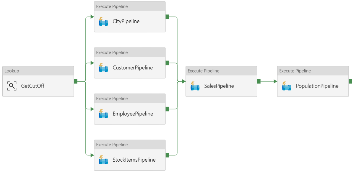
In Azure Data Factory, a pipeline is a logical grouping of activities used to coordinate a task — in this case, loading and transforming data into Azure Synapse.

This reference architecture defines a parent pipeline that runs a sequence of child pipelines. Each child pipeline loads data into one or more data warehouse tables.

Recommendations

Incremental loading

When you run an automated ETL or ELT process, it's most efficient to load only the data that changed since the previous run. This is called an incremental load, as opposed to a full load that loads all the data. To perform an incremental load, you need a way to identify which data has changed. The most common approach is to use a high water mark value, which means tracking the latest value of some column in the source table, either a datetime column or a unique integer column.

Starting with SQL Server 2016, you can use temporal tables. These are system-versioned tables that keep a full history of data changes. The database engine automatically records the history of every change in a separate history table. You can query the historical data by adding a FOR SYSTEM_TIME clause to a query. Internally, the database engine queries the history table, but this is transparent to the application.

Temporal tables are useful for dimension data, which can change over time. Fact tables usually represent an immutable transaction such as a sale, in which case keeping the system version history doesn't make sense. Instead, transactions usually have a column that represents the transaction date, which can be used as the watermark value. For example, in the Wide World Importers OLTP database, the Sales.Invoices and Sales.InvoiceLines tables have a LastEditedWhen field that defaults to sysdatetime().

Here is the general flow for the ELT pipeline:

1. For each table in the source database, track the cutoff time when the last ELT job ran. Store this information in the data warehouse. (On initial setup, all times are set to '1-1-1900'.)

2. During the data export step, the cutoff time is passed as a parameter to a set of stored procedures in the source database. These stored procedures query for any records that were changed or created after the cutoff time. For the Sales fact table, the LastEditedWhen column is used. For the dimension data, system-versioned temporal tables are used.

3. When the data migration is complete, update the table that stores the cutoff times.

It's also useful to record a lineage for each ELT run. For a given record, the lineage associates that record with the ELT run that produced the data. For each ETL run, a new lineage record is created for every table, showing the starting and ending load times. The lineage keys for each record are stored in the dimension and fact tables.

After a new batch of data is loaded into the warehouse, refresh the Analysis Services tabular model. See Asynchronous refresh with the REST API.

Data cleansing

Data cleansing should be part of the ELT process. In this reference architecture, one source of bad data is the city population table, where some cities have zero population, perhaps because no data was available. During processing, the ELT pipeline removes those cities from the city population table. Perform data cleansing on staging tables, rather than external tables.

External data sources

Data warehouses often consolidate data from multiple sources. For example, an external data source that contains demographics data. This dataset is available in Azure blob storage as part of the WorldWideImportersDW sample.

Azure Data Factory can copy directly from blob storage, using the blob storage connector. However, the connector requires a connection string or a shared access signature, so it can't be used to copy a blob with public read access. As a workaround, you can use PolyBase to create an external table over Blob storage and then copy the external tables into Azure Synapse.

Handling large binary data

For example, in the source database, a City table has a Location column that holds a geography spatial data type. Azure Synapse doesn't support the geography type natively, so this field is converted to a varbinary type during loading. (See Workarounds for unsupported data types.)

However, PolyBase supports a maximum column size of varbinary(8000), which means some data could be truncated. A workaround for this problem is to break the data up into chunks during export, and then reassemble the chunks, as follows:

1. Create a temporary staging table for the Location column.

2. For each city, split the location data into 8000-byte chunks, resulting in 1 – N rows for each city.

3. To reassemble the chunks, use the T-SQL PIVOT operator to convert rows into columns and then concatenate the column values for each city.

The challenge is that each city will be split into a different number of rows, depending on the size of geography data. For the PIVOT operator to work, every city must have the same number of rows. To make this work, the T-SQL query does some tricks to pad out the rows with blank values, so that every city has the same number of columns after the pivot. The resulting query turns out to be much faster than looping through the rows one at a time.

The same approach is used for image data.

Slowly changing dimensions

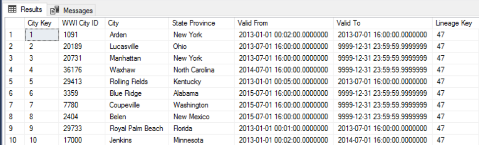
Dimension data is relatively static, but it can change. For example, a product might get reassigned to a different product category. There are several approaches to handling slowly changing dimensions. A common technique, called Type 2, is to add a new record whenever a dimension changes.

In order to implement the Type 2 approach, dimension tables need additional columns that specify the effective date range for a given record. Also, primary keys from the source database will be duplicated, so the dimension table must have an artificial primary key.

For example, the following image shows the Dimension.City table. The WWI City ID column is the primary key from the source database. The City Key column is an artificial key generated during the ETL pipeline. Also notice that the table has Valid From and Valid To columns, which define the range when each row was valid. Current values have a Valid To equal to '9999-12-31'.

The advantage of this approach is that it preserves historical data, which can be valuable for analysis. However, it also means there will be multiple rows for the same entity. For example, here are the records that match WWI City ID = 28561:

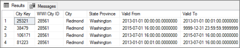
For each Sales fact, you want to associate that fact with a single row in City dimension table, corresponding to the invoice date.

Considerations

These considerations implement the pillars of the Azure Well-Architected Framework, which is a set of guiding tenets that can be used to improve the quality of a workload. For more information, see Microsoft Azure Well-Architected Framework.

Security

Security provides assurances against deliberate attacks and the abuse of your valuable data and systems. For more information, see Overview of the security pillar.

For additional security, you can use Virtual Network service endpoints to secure Azure service resources to only your virtual network. This fully removes public Internet access to those resources, allowing traffic only from your virtual network.

With this approach, you create a VNet in Azure and then create private service endpoints for Azure services. Those services are then restricted to traffic from that virtual network. You can also reach them from your on-premises network through a gateway.

Be aware of the following limitations:

• If service endpoints are enabled for Azure Storage, PolyBase cannot copy data from Storage into Azure Synapse. There is a mitigation for this issue. For more information, see Impact of using VNet Service Endpoints with Azure storage.

• To move data from on-premises into Azure Storage, you will need to allow public IP addresses from your on-premises or ExpressRoute. For details, see Securing Azure services to virtual networks.

• To enable Analysis Services to read data from Azure Synapse, deploy a Windows VM to the virtual network that contains the Azure Synapse service endpoint. Install Azure On-premises Data Gateway on this VM. Then connect your Azure Analysis service to the data gateway.

DevOps

• Create separate resource groups for production, development, and test environments. Separate resource groups make it easier to manage deployments, delete test deployments, and assign access rights.

• Put each workload in a separate deployment template and store the resources in source control systems. You can deploy the templates together or individually as part of a CI/CD process, making the automation process easier.

  In this architecture, there are three main workloads:

  • The data warehouse server, Analysis Services, and related resources.
  • Azure Data Factory.
  • An on-premises to cloud simulated scenario.

  Each workload has its own deployment template.

  The data warehouse server is set up and configured by using Azure CLI commands which follows the imperative approach of the IaC practice. Consider using deployment scripts and integrate them in the automation process.

• Consider staging your workloads. Deploy to various stages and run validation checks at each stage before moving to the next stage. That way you can push updates to your production environments in a highly controlled way and minimize unanticipated deployment issues. Use Blue-green deployment and Canary releases strategies for updating live production environments.

  Have a good rollback strategy for handling failed deployments. For example, you can automatically redeploy an earlier, successful deployment from your deployment history. See the --rollback-on-error flag parameter in Azure CLI.

• Azure Monitor is the recommended option for analyzing the performance of your data warehouse and the entire Azure analytics platform for an integrated monitoring experience. Azure Synapse Analytics provides a monitoring experience within the Azure portal to show insights to your data warehouse workload. The Azure portal is the recommended tool when monitoring your data warehouse because it provides configurable retention periods, alerts, recommendations, and customizable charts and dashboards for metrics and logs.

For more information, see the DevOps section in Microsoft Azure Well-Architected Framework.

Cost optimization

Cost optimization is about looking at ways to reduce unnecessary expenses and improve operational efficiencies. For more information, see Overview of the cost optimization pillar.

Use the Azure pricing calculator to estimate costs. Here are some considerations for services used in this reference architecture.

Azure Data Factory

Azure Data Factory automates the ELT pipeline. The pipeline moves the data from an on-premises SQL Server database into Azure Synapse. The data is then transformed into a tabular model for analysis. For this scenario, pricing starts from $ 0.001 activity runs per month that includes activity, trigger, and debug runs. That price is the base charge only for orchestration. You are also charged for execution activities, such as copying data, lookups, and external activities. Each activity is individually priced. You are also charged for pipelines with no associated triggers or runs within the month. All activities are prorated by the minute and rounded up.

Example cost analysis

Consider a use case where there are two lookups activities from two different sources. One takes 1 minute and 2 seconds (rounded up to 2 minutes) and the other one takes 1 minute resulting in total time of 3 minutes. One data copy activity takes 10 minutes. One stored procedure activity takes 2 minutes. Total activity runs for 4 minutes. Cost is calculated as follows:

Activity runs: 4 * $ 0.001 = $0.004

Lookups: 3 * ($0.005 / 60) = $0.00025

Stored procedure: 2 * ($0.00025 / 60) = $0.000008

Data copy: 10 * ($0.25 / 60) * 4 data integration unit (DIU) = $0.167

• Total cost per pipeline run: $0.17.
• Run once per day for 30 days: $5.1 month.
• Run once per day per 100 tables for 30 days: $ 510

Every activity has an associated cost. Understand the pricing model and use the ADF pricing calculator to get a solution optimized not only for performance but also for cost. Manage your costs by starting, stopping, pausing, and scaling your services.

Azure Synapse

Azure Synapse is ideal for intensive workloads with higher query performance and compute scalability needs. You can choose the pay-as-you-go model or use reserved plans of one year (37% savings) or 3 years (65% savings).

Data storage is charged separately. Other services such as disaster recovery and threat detection are also charged separately.

For more information, see Azure Synapse Pricing.

Analysis Services

Pricing for Azure Analysis Services depends on the tier. The reference implementation of this architecture uses the Developer tier, which is recommended for evaluation, development, and test scenarios. Other tiers include, the Basic tier, which is recommended for small production environment; the Standard tier for mission-critical production applications. For more information, see The right tier when you need it.

No charges apply when you pause your instance.

For more information, see Azure Analysis Services pricing.

Blob Storage

Consider using the Azure Storage reserved capacity feature to lower cost on storage. With this model, you get a discount if you can commit to reservation for fixed storage capacity for one or three years. For more information, see Optimize costs for Blob storage with reserved capacity.

For more information, see the Cost section in Microsoft Azure Well-Architected Framework.

Next steps

• Introduction to Azure Synapse Analytics
• Get Started with Azure Synapse Analytics
• Introduction to Azure Data Factory
• What is Azure Data Factory?
• Azure Data Factory tutorials

Related resources

You may want to review the following Azure example scenarios that demonstrate specific solutions using some of the same technologies:

• Data warehousing and analytics for sales and marketing
• Enterprise BI in Azure with Azure Synapse.