Generalized Linear Models using RevoScaleR
Important
This content is being retired and may not be updated in the future. The support for Machine Learning Server will end on July 1, 2022. For more information, see What's happening to Machine Learning Server?
Generalized linear models (GLM) are a framework for a wide range of analyses. They relax the assumptions for a standard linear model in two ways. First, a functional form can be specified for the conditional mean of the predictor, referred to as the “link” function. Second, you can specify a distribution for the response variable. The rxGlm function in RevoScaleR provides the ability to estimate generalized linear models on large data sets.
The following family/link combinations are implemented in C++ for performance enhancements: binomial/logit, gamma/log, poisson/log, and Tweedie. Other family/link combinations use a combination of C++ and R code. Any valid R family object that can be used with glm() can be used with rxGlm(), including user-defined. The following table shows all of the supported family/link combinations (in addition to user-defined):
| Family | Default Link Function | Other Available Link Functions |
|---|---|---|
| binomial | "logit" | "probit", "cauchit", "log", "cloglog" |
| gaussian | "identity" | "log", "inverse" |
| Gamma | "inverse" | "identity", "log" |
| inverse.gaussian | "1/mu^2" | "inverse", "identity", "log" |
| poisson | "log" | "identity", "sqrt" |
| quasi | "identity" with variance = "constant" | "logit", "probit", "cloglog", "inverse", "log", "1/mu^2", "sqrt" |
| quasibinomial | "logit" | Same as binomial, but dispersion parameter not fixed at one |
| quasipoisson | "log" | Same as poisson, but dispersion parameter not fixed at one |
| rxTweedie | requires arguments instead of link function |
A Simple Example Using the Poisson Family
The Poisson family is used to estimate models of count data. Examples from the literature include the following types of response variables:
- Number of drinks on a Saturday night
- Number of bacterial colonies in a Petri dish
- Number of children born to married women
- Number of credit cards a person has
We’ll start with a simple example from Kabacoff’s R in Action book, using data provided with the robust R package. The data are from a placebo-controlled clinical trial of 59 epileptics. Patients with partial seizures were enrolled in a randomized clinical trial of the anti-epileptic drug, progabide. Counts of epileptic seizures were recorded during the trial. The data set also includes a baseline 8-week seizure count and the age of the patient.
To access this data, first make sure the robust package is installed, then use the data command to load the data frame:
#  A Simple Example Using the Poisson Family

if ("robust" %in% .packages()){
data(breslow.dat, package = "robust")
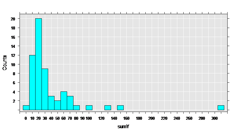
First, let’s get some basic information on the data set, then draw a histogram of the sumY variable, containing the total count of seizures during the trial.
rxGetInfo(breslow.dat, getVarInfo = TRUE)
rxHistogram( ~sumY, numBreaks = 25, data = breslow.dat)
The data set has 59 observations, and 12 variables. The variables of interest are Base, Age, Trt, and sumY.
Data frame: breslow.dat
Number of observations: 59
Number of variables: 12
Variable information:
Var 1: ID, Type: integer, Low/High: (101, 238)
Var 2: Y1, Type: integer, Low/High: (0, 102)
Var 3: Y2, Type: integer, Low/High: (0, 65)
Var 4: Y3, Type: integer, Low/High: (0, 76)
Var 5: Y4, Type: integer, Low/High: (0, 63)
Var 6: Base, Type: integer, Low/High: (6, 151)
Var 7: Age, Type: integer, Low/High: (18, 42)
Var 8: Trt
		2 factor levels: placebo progabide
Var 9: Ysum, Type: integer, Low/High: (0, 302)
Var 10: sumY, Type: integer, Low/High: (0, 302)
Var 11: Age10, Type: numeric, Low/High: (1.8000, 4.2000)
Var 12: Base4, Type: numeric, Low/High: (1.5000, 37.7500)
To estimate a model with sumY as the response variable and the Base number of seizures, Age, and the treatment as explanatory variables, we can use rxGlm. A benefit to using rxGlm is that the code scales for use with a much bigger data set.
myGlm <- rxGlm(sumY~ Base + Age + Trt, dropFirst = TRUE,
	data = breslow.dat, family = poisson())
summary(myGlm)
Results in:
Call:
rxGlm(formula = sumY ~ Base + Age + Trt, data = breslow.dat,
	family = poisson(), dropFirst = TRUE)

Generalized Linear Model Results for: sumY ~ Base + Age + Trt
Data: breslow.dat
Dependent variable(s): sumY
Total independent variables: 5 (Including number dropped: 1)
Number of valid observations: 59
Number of missing observations: 0
Family-link: poisson-log

Residual deviance: 559.4437 (on 55 degrees of freedom)

Coefficients:
				Estimate Std. Error t value Pr(>|t|)
(Intercept)    1.9488259  0.1356191  14.370 2.22e-16 ***
Base           0.0226517  0.0005093  44.476 2.22e-16 ***
Age            0.0227401  0.0040240   5.651 5.85e-07 ***
Trt=placebo      Dropped    Dropped Dropped  Dropped
Trt=progabide -0.1527009  0.0478051  -3.194  0.00232 **
---
Signif. codes:  0 '***' 0.001 '**' 0.01 '*' 0.05 '.' 0.1 ' ' 1

(Dispersion parameter for poisson family taken to be 1)

Condition number of final variance-covariance matrix: 3.3382
Number of iterations: 4
To interpret the coefficients, it is sometimes useful to transform them back to the original scale of the dependent variable. In this case:
exp(coef(myGlm))

	(Intercept)          Base           Age   Trt=placebo Trt=progabide
	7.0204403     1.0229102     1.0230007            NA     0.8583864
This suggests that, controlling for the base number of seizures and age, people taking progabide during the trial had 85% of the expected number seizures compared with people who didn’t.
A common method of checking for overdispersion is to calculate the ratio of the residual deviance with the degrees of freedom. This should be about 1 to fit the assumptions of the model.
myGlm$deviance/myGlm$df[2]

	[1] 10.1717
We can see that the ratio is well above one.
The quasi-poisson family can be used to handle over-dispersion. In this case, instead of assuming that the variance and mean are one, a relationship is estimated from the data:
myGlm1 <- rxGlm(sumY ~ Base + Age + Trt, dropFirst = TRUE,
	data = breslow.dat, family = quasipoisson())

summary(myGlm1)
} # End of if for robust package

	Call:
	rxGlm(formula = sumY ~ Base + Age + Trt, data = breslow.dat,
		family = quasipoisson(), dropFirst = TRUE)

	Generalized Linear Model Results for: sumY ~ Base + Age + Trt
	Data: breslow.dat
	Dependent variable(s): sumY
	Total independent variables: 5 (Including number dropped: 1)
	Number of valid observations: 59
	Number of missing observations: 0
	Family-link: quasipoisson-log

	Residual deviance: 559.4437 (on 55 degrees of freedom)

	Coefficients:
					Estimate Std. Error t value Pr(>|t|)
	(Intercept)    1.948826   0.465091   4.190 0.000102 ***
	Base           0.022652   0.001747  12.969 2.22e-16 ***
	Age            0.022740   0.013800   1.648 0.105085
	Trt=placebo     Dropped    Dropped Dropped  Dropped
	Trt=progabide -0.152701   0.163943  -0.931 0.355702
	---
	Signif. codes:  0 '***' 0.001 '**' 0.01 '*' 0.05 '.' 0.1 ' ' 1

	(Dispersion parameter for quasipoisson family taken to be 11.76075)

	Condition number of final variance-covariance matrix: 3.3382
	Number of iterations: 4
Notice that the coefficients are the same as when using the poisson family, but that the standard errors are larger. The effect of the treatment is no longer significant.
An Example Using the Gamma Family
The Gamma family is used with data containing positive values with a positive skew. A classic example is estimating the value of auto insurance claims. Using the sample claims.xdf data set:
#  An Example Using the Gamma Family

claimsXdf <- file.path(rxGetOption("sampleDataDir"),"claims.xdf")

claimsGlm <- rxGlm(cost ~ age + car.age + type, family = Gamma,
				dropFirst = TRUE, data = claimsXdf)
summary(claimsGlm)

	Call:
	rxGlm(formula = cost ~ age + car.age + type, data = claimsXdf,
		family = Gamma, dropFirst = TRUE)

	Generalized Linear Model Results for: cost ~ age + car.age + type
	File name:
		C:\Program Files\Microsoft\MRO-for-RRE\8.0\R-3.2.2\library\RevoScaleR\SampleData\claims.xdf
	Dependent variable(s): cost
	Total independent variables: 17 (Including number dropped: 3)
	Number of valid observations: 123
	Number of missing observations: 5
	Family-link: Gamma-inverse

	Residual deviance: 15.6397 (on 109 degrees of freedom)

	Coefficients:
				Estimate Std. Error t value Pr(>|t|)
	(Intercept)  0.0032807  0.0005126   6.400 4.02e-09 ***
	age=17-20      Dropped    Dropped Dropped  Dropped
	age=21-24    0.0006593  0.0005471   1.205 0.230843
	age=25-29    0.0003911  0.0005183   0.755 0.452114
	age=30-34    0.0012388  0.0005982   2.071 0.040720 *
	age=35-39    0.0017152  0.0006514   2.633 0.009685 **
	age=40-49    0.0012649  0.0006007   2.106 0.037516 *
	age=50-59    0.0002863  0.0005087   0.563 0.574771
	age=60+      0.0013006  0.0006041   2.153 0.033519 *
	car.age=0-3    Dropped    Dropped Dropped  Dropped
	car.age=4-7  0.0003444  0.0003535   0.974 0.332120
	car.age=8-9  0.0011005  0.0004161   2.645 0.009375 **
	car.age=10+  0.0034437  0.0006107   5.639 1.36e-07 ***
	type=A         Dropped    Dropped Dropped  Dropped
	type=B      -0.0004443  0.0004880  -0.911 0.364508
	type=C      -0.0004189  0.0004912  -0.853 0.395668
	type=D      -0.0016209  0.0004344  -3.732 0.000304 ***
	---
	Signif. codes:  0 '***' 0.001 '**' 0.01 '*' 0.05 '.' 0.1 ' ' 1

	(Dispersion parameter for Gamma family taken to be 0.1785316)

	Condition number of final variance-covariance matrix: 12.4648
	Number of iterations: 4
But, these estimates are conditional on the fact that a claim was made.
An Example Using the Tweedie Family
The Tweedie family of distributions provides flexible models for estimation. The power parameter var.power determines the shape of the distribution, with familiar models as special cases: if var.power is set to 0, Tweedie is a normal distribution; when set to 1, it is Poisson; when 2, it is Gamma; when 3, it is inverse Gaussian. If var.power is between 1 and 2, it is a compound Poisson distribution and is appropriate for positive data that also contains exact zeros, for example, insurance claims data, rainfall data, or fish-catch data. If var.power is greater than 2, it is appropriate for positive data.
In this example, we use a subsample from the 5% sample of the U.S. 2000 census. We consider the annual cost of property insurance for heads of household ages 21 through 89, and its relationship to age, sex, and region. A variable “perwt” in the data set represents the probability weight for that observation. First, to create the subsample (specify the correct data path for your downloaded data):
bigDataDir = "C:/MRS/Data"
bigCensusData <- file.path(bigDataDir, "Census5PCT2000.xdf")
propinFile <- "CensusPropertyIns.xdf"

propinDS <- rxDataStep(inData = bigCensusData, outFile = propinFile,
	rowSelection =  (related == 'Head/Householder') & (age > 20) & (age < 90),
	varsToKeep = c("propinsr", "age", "sex", "region", "perwt"),
	blocksPerRead = 10, overwrite = TRUE)
rxGetInfo(propinDS)

	File name: C:\YourWorkingDir\CensusPropertyIns.xdf
	Number of observations: 5175270
	Number of variables: 5
	Number of blocks: 10
	Compression type: zlib
The
blocksPerReadargument is ignored when run locally using R Client. Learn more...
An Xdf data source representing the new data file is returned. The new data file has over 5 million observations.
Let’s do one more step in data cleaning. The variable region has some long factor level character strings, and it also has a number of levels for which there are no observations. We can see this using rxSummary:
rxSummary(~region, data = propinDS)

	Call:
	rxSummary(formula = ~region, data = propinDS)

	Summary Statistics Results for: ~region
	File name: C:\YourWorkingDir\CensusPropertyIns.xdf
	Number of valid observations: 5175270


	Category Counts for region
	Number of categories: 17
	Number of valid observations: 5175270
	Number of missing observations: 0

	region                                           Counts
	New England Division                             265372
	Middle Atlantic Division                         734585
	Mixed Northeast Divisions (1970 Metro)                0
	East North Central Div.                          847367
	West North Central Div.                          366417
	Mixed Midwest Divisions (1970 Metro)                  0
	South Atlantic Division                          981614
	East South Central Div.                          324003
	West South Central Div.                          553425
	Mixed Southern Divisions (1970 Metro)                 0
	Mountain Division                                328940
	Pacific Division                                 773547
	Mixed Western Divisions (1970 Metro)                  0
	Military/Military reservations                        0
	PUMA boundaries cross state lines-1% sample           0
	State not identified                                  0
	Inter-regional county group (1970 Metro samples)      0
We can use the rxFactors function rename and reduce the number of levels:
regionLevels <- list( "New England" = "New England Division",
	"Middle Atlantic" = "Middle Atlantic Division",
	"East North Central" = "East North Central Div.",
	"West North Central" = "West North Central Div.",
	"South Atlantic" = "South Atlantic Division",
	"East South Central" = "East South Central Div.",
	"West South Central" = "West South Central Div.",
	"Mountain" ="Mountain Division",
	"Pacific" ="Pacific Division")

rxFactors(inData = propinDS, outFile = propinDS,
	factorInfo = list(region = list(newLevels = regionLevels,
		otherLevel = "Other")),
	overwrite = TRUE)
As a first step to analysis, let’s look at a histogram of the property insurance cost:
rxHistogram(~propinsr, data = propinDS, pweights = "perwt")
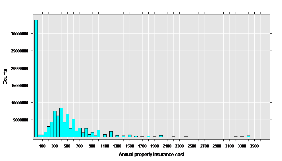
This data appears to be a good match for the Tweedie family with a variance power parameter between 1 and 2, since it has a “clump” of exact zeros in addition to a distribution of positive values.
We can estimate the parameters using rxGlm, setting the var.power argument to 1.5. As explanatory variables we’ll use sex, an “on-the-fly” factor variable with a level for each age, and region:
propinGlm <- rxGlm(propinsr~sex + F(age) + region,
pweights = "perwt", data = propinDS,
family = rxTweedie(var.power = 1.5), dropFirst = TRUE)
summary(propinGlm)

Call:
rxGlm(formula = propinsr ~ sex + F(age) + region, data = propinDS,
family = rxTweedie(var.power = 1.5), pweights = "perwt",
dropFirst = TRUE)

Generalized Linear Model Results for: propinsr ~ sex + F(age) + region
File name: C:\YourWorkingDir\CensusPropertyIns.xdf
Probability weights: perwt
Dependent variable(s): propinsr
Total independent variables: 82 (Including number dropped: 4)
Number of valid observations: 5175270
Number of missing observations: 0
Family-link: Tweedie-mu^-0.5

Residual deviance: 3292809839.3236 (on 5175192 degrees of freedom)

Coefficients:
						Estimate Std. Error  t value Pr(>|t|)
(Intercept)                1.231e-01  5.893e-04  208.961 2.22e-16 ***
sex=Male                     Dropped    Dropped  Dropped  Dropped
sex=Female                 9.026e-03  3.164e-05  285.305 2.22e-16 ***
F_age=21                     Dropped    Dropped  Dropped  Dropped
F_age=22                  -9.208e-03  7.523e-04  -12.240 2.22e-16 ***
F_age=23                  -1.980e-02  6.966e-04  -28.430 2.22e-16 ***
F_age=24                  -2.856e-02  6.648e-04  -42.955 2.22e-16 ***
F_age=25                  -3.652e-02  6.432e-04  -56.776 2.22e-16 ***
F_age=26                  -4.371e-02  6.289e-04  -69.500 2.22e-16 ***
F_age=27                  -4.894e-02  6.182e-04  -79.162 2.22e-16 ***
F_age=28                  -5.398e-02  6.099e-04  -88.506 2.22e-16 ***
F_age=29                  -5.787e-02  6.043e-04  -95.749 2.22e-16 ***
F_age=30                  -6.064e-02  6.020e-04 -100.716 2.22e-16 ***
F_age=31                  -6.336e-02  6.004e-04 -105.522 2.22e-16 ***
F_age=32                  -6.526e-02  5.991e-04 -108.933 2.22e-16 ***
F_age=33                  -6.721e-02  5.975e-04 -112.489 2.22e-16 ***
F_age=34                  -6.854e-02  5.962e-04 -114.948 2.22e-16 ***
F_age=35                  -6.942e-02  5.949e-04 -116.688 2.22e-16 ***
F_age=36                  -7.090e-02  5.941e-04 -119.342 2.22e-16 ***
F_age=37                  -7.184e-02  5.936e-04 -121.023 2.22e-16 ***
F_age=38                  -7.265e-02  5.931e-04 -122.498 2.22e-16 ***
F_age=39                  -7.354e-02  5.926e-04 -124.090 2.22e-16 ***
F_age=40                  -7.401e-02  5.923e-04 -124.954 2.22e-16 ***
F_age=41                  -7.462e-02  5.923e-04 -125.994 2.22e-16 ***
F_age=42                  -7.508e-02  5.920e-04 -126.819 2.22e-16 ***
F_age=43                  -7.568e-02  5.920e-04 -127.846 2.22e-16 ***
F_age=44                  -7.597e-02  5.919e-04 -128.344 2.22e-16 ***
F_age=45                  -7.642e-02  5.918e-04 -129.139 2.22e-16 ***
F_age=46                  -7.693e-02  5.919e-04 -129.973 2.22e-16 ***
F_age=47                  -7.727e-02  5.918e-04 -130.564 2.22e-16 ***
F_age=48                  -7.749e-02  5.919e-04 -130.927 2.22e-16 ***
F_age=49                  -7.783e-02  5.919e-04 -131.488 2.22e-16 ***
F_age=50                  -7.809e-02  5.919e-04 -131.941 2.22e-16 ***
F_age=51                  -7.853e-02  5.919e-04 -132.678 2.22e-16 ***
F_age=52                  -7.888e-02  5.916e-04 -133.326 2.22e-16 ***
F_age=53                  -7.919e-02  5.916e-04 -133.859 2.22e-16 ***
F_age=54                  -7.909e-02  5.931e-04 -133.348 2.22e-16 ***
F_age=55                  -7.938e-02  5.929e-04 -133.873 2.22e-16 ***
F_age=56                  -7.930e-02  5.929e-04 -133.751 2.22e-16 ***
F_age=57                  -7.959e-02  5.928e-04 -134.276 2.22e-16 ***
F_age=58                  -7.935e-02  5.937e-04 -133.644 2.22e-16 ***
F_age=59                  -7.923e-02  5.942e-04 -133.336 2.22e-16 ***
F_age=60                  -7.894e-02  5.946e-04 -132.753 2.22e-16 ***
F_age=61                  -7.917e-02  5.947e-04 -133.122 2.22e-16 ***
F_age=62                  -7.912e-02  5.949e-04 -133.003 2.22e-16 ***
F_age=63                  -7.904e-02  5.954e-04 -132.746 2.22e-16 ***
F_age=64                  -7.886e-02  5.956e-04 -132.405 2.22e-16 ***
F_age=65                  -7.878e-02  5.952e-04 -132.359 2.22e-16 ***
F_age=66                  -7.871e-02  5.961e-04 -132.031 2.22e-16 ***
F_age=67                  -7.864e-02  5.963e-04 -131.869 2.22e-16 ***
F_age=68                  -7.861e-02  5.966e-04 -131.766 2.22e-16 ***
F_age=69                  -7.845e-02  5.967e-04 -131.490 2.22e-16 ***
F_age=70                  -7.861e-02  5.965e-04 -131.790 2.22e-16 ***
F_age=71                  -7.856e-02  5.970e-04 -131.600 2.22e-16 ***
F_age=72                  -7.850e-02  5.971e-04 -131.460 2.22e-16 ***
F_age=73                  -7.813e-02  5.977e-04 -130.714 2.22e-16 ***
F_age=74                  -7.818e-02  5.981e-04 -130.722 2.22e-16 ***
F_age=75                  -7.800e-02  5.986e-04 -130.302 2.22e-16 ***
F_age=76                  -7.781e-02  5.993e-04 -129.825 2.22e-16 ***
F_age=77                  -7.763e-02  6.002e-04 -129.342 2.22e-16 ***
F_age=78                  -7.735e-02  6.009e-04 -128.728 2.22e-16 ***
F_age=79                  -7.724e-02  6.024e-04 -128.221 2.22e-16 ***
F_age=80                  -7.646e-02  6.045e-04 -126.495 2.22e-16 ***
F_age=81                  -7.651e-02  6.060e-04 -126.244 2.22e-16 ***
F_age=82                  -7.643e-02  6.081e-04 -125.693 2.22e-16 ***
F_age=83                  -7.600e-02  6.109e-04 -124.411 2.22e-16 ***
F_age=84                  -7.546e-02  6.145e-04 -122.798 2.22e-16 ***
F_age=85                  -7.529e-02  6.183e-04 -121.775 2.22e-16 ***
F_age=86                  -7.441e-02  6.259e-04 -118.882 2.22e-16 ***
F_age=87                  -7.422e-02  6.324e-04 -117.363 2.22e-16 ***
F_age=88                  -7.339e-02  6.463e-04 -113.553 2.22e-16 ***
F_age=89                  -7.310e-02  6.569e-04 -111.284 2.22e-16 ***
region=New England           Dropped    Dropped  Dropped  Dropped
region=Middle Atlantic     1.710e-03  6.893e-05   24.807 2.22e-16 ***
region=East North Central  3.552e-03  6.867e-05   51.723 2.22e-16 ***
region=West North Central  4.200e-04  7.697e-05    5.457 4.83e-08 ***
region=South Atlantic     -1.227e-03  6.521e-05  -18.821 2.22e-16 ***
region=East South Central -7.894e-04  7.793e-05  -10.130 2.22e-16 ***
region=West South Central -5.857e-03  6.732e-05  -87.011 2.22e-16 ***
region=Mountain            1.821e-03  8.060e-05   22.596 2.22e-16 ***
region=Pacific            -5.990e-04  6.732e-05   -8.897 2.22e-16 ***
region=Other                 Dropped    Dropped  Dropped  Dropped
---
Signif. codes:  0 '***' 0.001 '**' 0.01 '*' 0.05 '.' 0.1 ' ' 1

(Dispersion parameter for Tweedie family taken to be 546.4888)

Condition number of final variance-covariance matrix: 5980.277
Number of iterations: 8
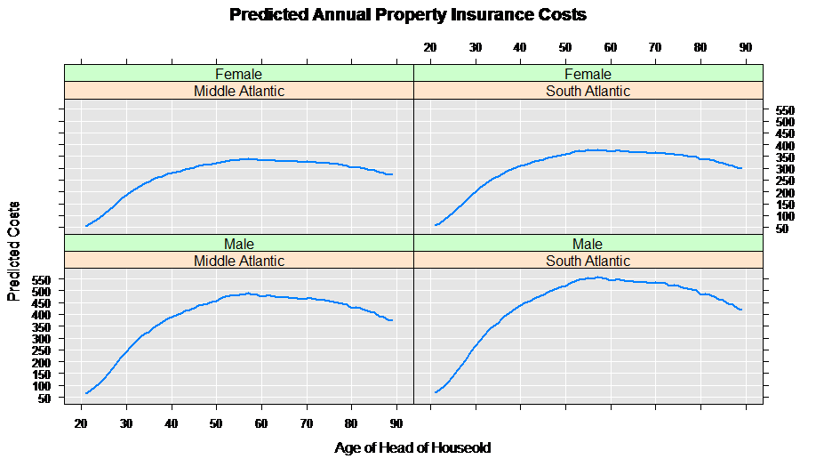
A good way to begin examining the results of the estimated model is to look at predicted values for given explanatory characteristics. For example, let’s create a prediction data set for the South Atlantic region for all ages and sexes:
# Get the region factor levels
varInfo <- rxGetVarInfo(propinDS)
regionLabels <- varInfo$region$levels

# Create a prediction data set for region 5, all ages, both sexes
region <- factor(rep(5, times=138), levels = 1:10, labels = regionLabels)
age <- c(21:89, 21:89)
sex <- factor(c(rep(1, times=69), rep(2, times=69)),
	levels = 1:2,
	labels = c("Male", "Female"))
predData <- data.frame(age, sex, region)
Now we’ll use that as a basis for a similar prediction data set for the Middle Atlantic region:
# Create a prediction data set for region 2, all ages, both sexes
predData2 <- predData
predData2$region <-factor(rep(2, times=138), levels = 1:10,
	labels = varInfo$region$levels)
Next we combine the two data sets, and compute the predicted values for annual property insurance cost using our estimated rxGlm model:
predData$predicted <- outData$propinsr_Pred
rxLinePlot( predicted ~age|region+sex, data = predData,
	title = "Predicted Annual Property Insurance Costs",
	xTitle = "Age of Head of Household",
	yTitle = "Predicted Costs")
Stepwise Generalized Linear Models
Stepwise generalized linear models help you determine which variables are most important to include in the model. You provide a minimal, or lower, model formula and a maximal, or upper, model formula. Using forward selection, backward elimination, or bidirectional search, the algorithm determines the model formula that provides the best fit based on an AIC selection criterion or a significance level criterion.
As an example, consider again the Gamma family model from earlier in this article:
claimsXdf <- file.path(rxGetOption("sampleDataDir"),"claims.xdf")
claimsGlm <- rxGlm(cost ~ age + car.age + type, family = Gamma,
				dropFirst = TRUE, data = claimsXdf)
summary(claimsGlm)
We can recast this model as a stepwise model by specifying a variableSelection argument using the rxStepControl function to provide our stepwise arguments:
claimsGlmStep <- rxGlm(cost ~ age, family = Gamma, dropFirst=TRUE,
					data=claimsXdf, variableSelection =
					rxStepControl(scope = ~ age + car.age + type ))
summary(claimsGlmStep)

	Call:
	rxGlm(formula = cost ~ age, data = claimsXdf, family = Gamma,
	variableSelection = rxStepControl(scope = ~age + car.age +
		type), dropFirst = TRUE)

	Generalized Linear Model Results for: cost ~ car.age + type
	File name:
	C:\Program Files\Microsoft\MRO-for-RRE\8.0\R-3.2.2\library\RevoScaleR\SampleData\claims.xdf
	Dependent variable(s): cost
	Total independent variables: 9 (Including number dropped: 2)
	Number of valid observations: 123
	Number of missing observations: 5
	Family-link: Gamma-inverse

	Residual deviance: 18.0433 (on 116 degrees of freedom)

	Coefficients:
				Estimate Std. Error t value Pr(>|t|)
	(Intercept)  0.0040354  0.0004661   8.657 3.24e-14 ***
	car.age=0-3    Dropped    Dropped Dropped  Dropped
	car.age=4-7  0.0003568  0.0004037   0.884  0.37868
	car.age=8-9  0.0011825  0.0004688   2.522  0.01302 *
	car.age=10+  0.0035478  0.0006853   5.177 9.57e-07 ***
	type=A         Dropped    Dropped Dropped  Dropped
	type=B      -0.0004512  0.0005519  -0.818  0.41528
	type=C      -0.0004135  0.0005558  -0.744  0.45837
	type=D      -0.0016307  0.0004923  -3.313  0.00123 **
	---
	Signif. codes:  0 ‘***’ 0.001 ‘**’ 0.01 ‘*’ 0.05 ‘.’ 0.1 ‘ ’ 1

	(Dispersion parameter for Gamma family taken to be 0.2249467)

	Condition number of final variance-covariance matrix: 9.1775
	Number of iterations: 5
We see that in the stepwise model fit, age no longer appears in the final model.
Plotting Model Coefficients
The ability to save model coefficients using the argument keepStepCoefs = TRUE within the rxStepControl call, and to plot them with the function rxStepPlot was described in great detail for stepwise rxLinMod in Fitting Linear Models using RevoScaleR. This functionality is also available for stepwise rxGLM objects.