Tutorial: Load and analyze a large airline data set with RevoScaleR

Artikel
11/03/2016

Important

This content is being retired and may not be updated in the future. The support for Machine Learning Server will end on July 1, 2022. For more information, see What's happening to Machine Learning Server?

This tutorial builds on what you learned in the first RevoScaleR tutorial by exploring the functions, techniques, and issues arising when working with larger data sets. As before, you'll work with sample data to complete the steps, except this time you will use a much larger data set.

Download the airline dataset

To really get a feel for RevoScaleR, you should work with functions using a larger data set. Larger data sets are available for download from this web page.

You can use a smaller or larger data set with this tutorial. Datasets for this tutorial include the following:

AirOnTime87to12: An .xdf file containing information on flight arrival and departure details for all commercial flights within the USA, from October 1987 to December 2012. This is a large dataset: there are nearly 150 million records in total. It is just under 4 GB unpacked.
AirOnTime7Pct: A 7% subsample of AirOnTimeData87to12. This is an .xdf file containing just the variables used in the examples in this tutorial. It can be used as an alternative. This subsample contains a little over 10 million rows of data. It is about 100 MB unpacked.

When downloading these files, put them in a directory where you can easily access them. For example, create a directory "C:\MRS\BigData" and unpack the files there. When running examples using these files, you will want to specify this location as your bigDataDir. For example:

bigDataDir <- "C:\MRS\BigData"

Origin of the sample datasets

Airline on-time performance data for the years 1987 through 2008 was used in the American Statistical Association Data Expo in 2009 (http://stat-computing.org/dataexpo/2009/). ASA describes the data set as follows:

The data consists of flight arrival and departure details for all commercial flights within the USA, from October 1987 to April 2008. This is a large dataset: there are nearly 120 million records in total, and takes up 1.6 gigabytes of space compressed and 12 gigabytes when uncompressed.

Data by month can be downloaded as comma-delimited text files from the Research and Innovative Technology Administration (RITA) of the Bureau of Transportation Statistics web site (http://www.transtats.bts.gov/DL_SelectFields.asp?Table_ID=236). Data from 1987 through 2012 has been imported into an .xdf file named AirOnTime87to12.xdf.

A much smaller subset containing 7% of the observations for the variables used in this example is also available as AirOnTime7Pct.xdf. This subsample contains a little over 10 million rows of data, so has about 60 times the rows of the smaller subsample used in the previous example. More information on this data set can be found in the help file: ?AirOnTime87to12. To view the help file, enter the file name at the > prompt in the R interactive window.

Explore the data

Assuming you specified a location of your downloaded data as the bigDataDir variable, create an object for the dataset as airDataName:

bigDataDir <- "C:/MRS/Data"

airDataName <- file.path(bigDataDir, "AirOnTime87to12")

airDataName <- file.path(bigDataDir,"AirOnTime7Pct")

Create an in-memory RxXdfObject data source object to represent the .xdf data file:

bigAirDS <- RxXdfData( airDataName )

Use the rxGetInfo function to get summary information on the active data set.

rxGetInfo(bigAirDS, getVarInfo=TRUE)

The full data set has 46 variables and almost 150 million observations.

File name: C:\MRS\Data\AirOnTime87to12\AirOnTime87to12.xdf
Number of observations: 148619655
Number of variables: 46
Number of blocks: 721
Compression type: zlib
Variable information:
Var 1: Year, Type: integer, Low/High: (1987, 2012)
Var 2: Month, Type: integer, Low/High: (1, 12)
Var 3: DayofMonth, Type: integer, Low/High: (1, 31)
Var 4: DayOfWeek
		7 factor levels: Mon Tues Wed Thur Fri Sat Sun
Var 5: FlightDate, Type: Date, Low/High: (1987-10-01, 2012-12-31)
Var 6: UniqueCarrier
		30 factor levels: AA US AS CO DL ... OH F9 YV 9E VX
Var 7: TailNum
		14463 factor levels: 0 N910DE N948DL N901DE N980DL ... N565UW N8326F N8327A N8328A N8329B
Var 8: FlightNum
		8206 factor levels: 1 2 3 5 6 ... 8546 9221 13 7413 8510
Var 9: OriginAirportID
		374 factor levels: 12478 12892 12173 13830 11298 ... 12335 12389 10466 14802 12888
Var 10: Origin
		373 factor levels: JFK LAX HNL OGG DFW ... IMT ISN AZA SHD LAR
Var 11: OriginState
		53 factor levels: NY CA HI TX MO ... SD DE PR VI TT
Var 12: DestAirportID
		378 factor levels: 12892 12173 12478 13830 11298 ... 11587 12335 12389 10466 14802
Var 13: Dest
		377 factor levels: LAX HNL JFK OGG DFW ... ESC IMT ISN AZA SHD
Var 14: DestState
		53 factor levels: CA HI NY TX MO ... WY DE PR VI TT
Var 15: CRSDepTime, Type: numeric, Storage: float32, Low/High: (0.0000, 24.0000)
Var 16: DepTime, Type: numeric, Storage: float32, Low/High: (0.0167, 24.0000)
Var 17: DepDelay, Type: integer, Low/High: (-1410, 2601)
Var 18: DepDelayMinutes, Type: integer, Low/High: (0, 2601)
Var 19: DepDel15, Type: logical, Low/High: (0, 1)
Var 20: DepDelayGroups
		15 factor levels: < -15 -15 to -1 0 to 14 15 to 29 30 to 44 ... 120 to 134 135 to 149 150 to 164 165 to 179 >= 180
Var 21: TaxiOut, Type: integer, Low/High: (0, 3905)
Var 22: WheelsOff, Type: numeric, Storage: float32, Low/High: (0.0000, 72.5000)
Var 23: WheelsOn, Type: numeric, Storage: float32, Low/High: (0.0000, 24.0000)
Var 24: TaxiIn, Type: integer, Low/High: (0, 1440)
Var 25: CRSArrTime, Type: numeric, Storage: float32, Low/High: (0.0000, 24.0000)
Var 26: ArrTime, Type: numeric, Storage: float32, Low/High: (0.0167, 24.0000)
Var 27: ArrDelay, Type: integer, Low/High: (-1437, 2598)
Var 28: ArrDelayMinutes, Type: integer, Low/High: (0, 2598)
Var 29: ArrDel15, Type: logical, Low/High: (0, 1)
Var 30: ArrDelayGroups
		15 factor levels: < -15 -15 to -1 0 to 14 15 to 29 30 to 44 ... 120 to
134 135 to 149 150 to 164 165 to 179 >= 180
Var 31: Cancelled, Type: logical, Low/High: (0, 1)
Var 32: CancellationCode
		5 factor levels: NA Carrier Weather NAS Security
Var 33: Diverted, Type: logical, Low/High: (0, 1)
Var 34: CRSElapsedTime, Type: integer, Low/High: (-162, 1865)
Var 35: ActualElapsedTime, Type: integer, Low/High: (-719, 1440)
Var 36: AirTime, Type: integer, Low/High: (-2378, 1399)
Var 37: Flights, Type: integer, Low/High: (1, 1)
Var 38: Distance, Type: integer, Low/High: (0, 4983)
Var 39: DistanceGroup
		11 factor levels: < 250 250-499 500-749 750-999 1000-1249 ... 1500-
1749 1750-1999 2000-2249 2250-2499 >= 2500
Var 40: CarrierDelay, Type: integer, Low/High: (0, 2580)
Var 41: WeatherDelay, Type: integer, Low/High: (0, 1615)
Var 42: NASDelay, Type: integer, Low/High: (-60, 1392)
Var 43: SecurityDelay, Type: integer, Low/High: (0, 782)
Var 44: LateAircraftDelay, Type: integer, Low/High: (0, 1407)
Var 45: MonthsSince198710, Type: integer, Low/High: (0, 302)
Var 46: DaysSince19871001, Type: integer, Low/High: (0, 9223)

Reading a Chunk of Data

Data stored in the xdf file format can be read into a data frame, allowing the user to choose the rows and columns. For example, read 1000 rows beginning at the 100,000th row for the variables ArrDelay, DepDelay, and DayOfWeek.

testDF <- rxDataStep(inData = bigAirDS,
	varsToKeep = c("ArrDelay","DepDelay", "DayOfWeek"),
	startRow = 100000, numRows = 1000)
summary(testDF)

You should see the following information if bigAirDS is the full data set, AirlineData87to08.xdf:

	        ArrDelay          DepDelay       DayOfWeek
	 Min.   :-65.000   Min.   : -5.000   Mon :138  
	 1st Qu.: -9.000   1st Qu.:  0.000   Tues:135  
	 Median : -2.000   Median :  0.000   Wed :136  
	 Mean   :  2.297   Mean   :  6.251   Thur:173  
	 3rd Qu.:  8.000   3rd Qu.:  1.000   Fri :168  
	 Max.   :262.000   Max.   :315.000   Sat :133  
	 NA's   :8         NA's   :3         Sun :117

And we can easily run a regression using the lm function in R using this small data set:

lmObj <- lm(ArrDelay~DayOfWeek, data = testDF)
summary(lmObj)

It yields the following:

Call:
lm(formula = ArrDelay ~ DayOfWeek, data = testDF)

Residuals:
	Min      1Q  Median      3Q     Max
-65.251 -12.131  -3.307   6.749 261.869

Coefficients:
				Estimate Std. Error t value Pr(>|t|)    
(Intercept)     0.1314     2.0149   0.065    0.948    
DayOfWeekTues   2.1074     2.8654   0.735    0.462    
DayOfWeekWed   -1.1981     2.8600  -0.419    0.675    
DayOfWeekThur   0.1201     2.7041   0.044    0.965    
DayOfWeekFri    0.7377     2.7149   0.272    0.786    
DayOfWeekSat   14.2302     2.8876   4.928 9.74e-07 ***
DayOfWeekSun    0.2874     2.9688   0.097    0.923    
---
Signif. codes:  0 ‘***’ 0.001 ‘**’ 0.01 ‘*’ 0.05 ‘.’ 0.1 ‘ ’ 1

Residual standard error: 23.58 on 985 degrees of freedom
	(8 observations deleted due to missingness)
Multiple R-squared:  0.03956,	Adjusted R-squared:  0.03371
F-statistic: 6.761 on 6 and 985 DF,  p-value: 4.91e-07

But this is only 1/148,619 of the rows contained in the full data set. If we try to read all the rows of these columns, we will likely run into memory problems. For example, on most systems with 8GB or less of RAM, running the commented code below will fail on the full data set with a "cannot allocate vector" error.

# testDF <- rxDataStep(inData=dataName, varsToKeep = c("ArrDelay",
#    "DepDelay", "DayOfWeek"))

In the next section you will see how you can analyze a data set that is too big to fit into memory by using RevoScaleR functions.

Estimating a Linear Model with a Huge Data Set

The RevoScaleR compute engine is designed to work very efficiently with .xdf files, particularly with factor data. When working with larger data sets, the blocksPerRead argument is important in controlling how much data is processed in memory at one time. If too many blocks are read in at one time, you may run out of memory. If too few blocks are read in at one time, you may experience slower total processing time. You can experiment with blocksPerRead on your system and time the estimation of a linear model as follows:

The blocksPerRead argument is ignored if run locally using R Client. Learn more...

system.time(
	delayArr <- rxLinMod(ArrDelay ~ DayOfWeek, data = bigAirDS,
		cube = TRUE, blocksPerRead = 30)
)

The linear model you get will not vary as you change blocksPerRead. To see a summary of your results:

summary(delayArr)

You should see the following results for the full data set:

Call:
rxLinMod(formula = ArrDelay ~ DayOfWeek, data = bigAirDS, cube = TRUE,
	blocksPerRead = 30)

Cube Linear Regression Results for: ArrDelay ~ DayOfWeek
File name: C:\MRS\Data\AirOnTime87to12\AirOnTime87to12.xdf
Dependent variable(s): ArrDelay
Total independent variables: 7
Number of valid observations: 145576737
Number of missing observations: 3042918

Coefficients:
				Estimate Std. Error t value Pr(>|t|)     |   Counts
DayOfWeek=Mon  6.365682   0.006810   934.7 2.22e-16 *** | 21414640
DayOfWeek=Tues 5.472585   0.006846   799.4 2.22e-16 *** | 21191074
DayOfWeek=Wed  6.538511   0.006832   957.1 2.22e-16 *** | 21280844
DayOfWeek=Thur 8.401000   0.006821  1231.7 2.22e-16 *** | 21349128
DayOfWeek=Fri  8.977519   0.006815  1317.3 2.22e-16 *** | 21386294
DayOfWeek=Sat  3.756762   0.007298   514.7 2.22e-16 *** | 18645919
DayOfWeek=Sun  6.062001   0.006993   866.8 2.22e-16 *** | 20308838
---
Signif. codes:  0 ‘***’ 0.001 ‘**’ 0.01 ‘*’ 0.05 ‘.’ 0.1 ‘ ’ 1

Residual standard error: 31.52 on 145576730 degrees of freedom
Multiple R-squared: 0.002585 (as if intercept included)
Adjusted R-squared: 0.002585
F-statistic: 6.289e+04 on 6 and 145576730 DF,  p-value: < 2.2e-16
Condition number: 1 1

Notice that because we specified cube = TRUE, we have an estimated coefficient for each day of the week (and not the intercept).

Because the computation is so fast, we can easily expand our analysis. For example, we can compare Arrival Delays with Departure Delays. First, we rerun the linear model, this time using Departure Delay as the dependent variable.

delayDep <- rxLinMod(DepDelay ~ DayOfWeek, data = bigAirDS,
	cube = TRUE, blocksPerRead = 30)

Next, combine the information from regression output in a data frame for plotting.

cubeResults <- rxResultsDF(delayArr)
cubeResults$DepDelay <- rxResultsDF(delayDep)$DepDelay

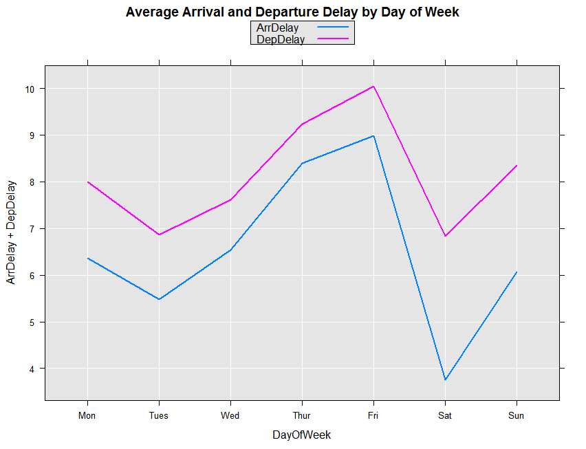
Then use the following code to plot the results, comparing the Arrival and Departure Delays by the Day of Week

rxLinePlot( ArrDelay + DepDelay ~ DayOfWeek, data = cubeResults,
	title = 'Average Arrival and Departure Delay by Day of Week')

You should see the following plot for the full data set:

DayOfWeek Plot

Turning Off Progress Reports

By default, RevoScaleR reports on the progress of the model fitting so that you can see that the computation is proceeding normally. You can specify an integer value from 0 through 3 to specify the level of reporting done; the default is 2. (See help on rxOptions to change the default.) For large model fits, this is usually reassuring. However, if you would like to turn off the progress reports, just use the argument reportProgress=0, which turns off reporting. For example, to suppress the progress reports in the estimation of the delayDep rxLinMod object, repeat the call as follows:

The blocksPerRead argument is ignored if run locally using R Client. Learn more...

delayDep <- rxLinMod(DepDelay ~ DayOfWeek, data = bigAirDS,
	cube = TRUE, blocksPerRead = 30, reportProgress = 0)

Handling Larger Linear Models

The data set contains a variable UniqueCarrier which contains airline codes for 29 carriers. Because the RevoScaleR Compute Engine handles factor variables so efficiently, we can do a linear regression looking at the Arrival Delay by Carrier. This will take a little longer, of course, than the previous analysis, because we are estimating 29 instead of 7 factor levels.

The blocksPerRead argument is ignored if run locally using R Client. Learn more...

delayCarrier <- rxLinMod(ArrDelay ~ UniqueCarrier,
	data = bigAirDS, cube = TRUE, blocksPerRead = 30)

Next, sort the coefficient vector so that the we can see the airlines with the highest and lowest values.

dcCoef <- sort(coef(delayCarrier))

Next, use the head function to show the top 10 with the lowest arrival delays:

head(dcCoef, 10)

In the full data set the result is:

	      UniqueCarrier=HA     UniqueCarrier=KH     UniqueCarrier=VX
	           -0.175857             1.156923             4.032345
	    UniqueCarrier=9E UniqueCarrier=ML (1)     UniqueCarrier=WN
	            4.362180             4.747609             5.070878
	UniqueCarrier=PA (1)     UniqueCarrier=OO     UniqueCarrier=NW
	            5.434067             5.453268             5.467372
	    UniqueCarrier=US
	            5.897604

Then use the tail function to show the bottom 10 with the highest arrival delays:

tail(dcCoef, 10)

With all of the data, you should see:

	UniqueCarrier=MQ UniqueCarrier=HP UniqueCarrier=OH UniqueCarrier=UA
	        7.563716         7.565358         7.801436         7.807771
	UniqueCarrier=YV UniqueCarrier=B6 UniqueCarrier=XE UniqueCarrier=PS
	        7.931515         8.154433         8.651180         9.261881
	UniqueCarrier=EV UniqueCarrier=PI
	        9.340071        10.464421

Notice that Hawaiian Airlines comes in as the best in on-time arrivals, while United is closer to the bottom of the list. We can see the difference by subtracting the coefficients:

sprintf("United's additional delay compared with Hawaiian: %f",
	dcCoef["UniqueCarrier=UA"]-dcCoef["UniqueCarrier=HA"])

which results in:

[1] "United's additional delay compared with Hawaiian: 7.983628"

Estimating Linear Models with Many Independent Variables

One ambitious question we could ask is to what extent the difference in delays is due to the differences in origins and destinations of the flights. To control for Origin and Destination we would need to add over 700 dummy variables in the full data set to represent the factor levels of Origin and Dest. The RevoScaleR Compute Engine is particularly efficient at handling this type of problem, so we can in fact run the regression:

The blocksPerRead argument is ignored if run locally using R Client. Learn more...

delayCarrierLoc <- rxLinMod(ArrDelay ~ UniqueCarrier + Origin+Dest,
	data = bigAirDS, cube = TRUE, blocksPerRead = 30)

dclCoef <- coef(delayCarrierLoc)
sprintf(
"United's additional delay accounting for dep and arr location: %f",
	dclCoef["UniqueCarrier=UA"]- dclCoef["UniqueCarrier=HA"])
paste("Number of coefficients estimated: ", length(!is.na(dclCoef)))

Accounting for origin and destination reduces the airline-specific difference in average delay:

[1] "United's additional delay accounting for dep and arr location: 2.045264"
[1] "Number of coefficients estimated:  780"

We can continue in this process, next adding variables to take account of the hour of day that the flight departed. Using the F function around the CRSDepTime will break the variable into factor categories, with one level for each hour of the day.

delayCarrierLocHour <- rxLinMod(ArrDelay ~
	UniqueCarrier + Origin + Dest + F(CRSDepTime),
	data = bigAirDS, cube = TRUE, blocksPerRead = 30)
dclhCoef <- coef(delayCarrierLocHour)

Now we can summarize all of our results:

sprintf("United's additional delay compared with Hawaiian: %f",
	dcCoef["UniqueCarrier=UA"]-dcCoef["UniqueCarrier=HA"])
paste("Number of coefficients estimated: ", length(!is.na(dcCoef)))
sprintf(
	"United's additional delay accounting for dep and arr location: %f",
	dclCoef["UniqueCarrier=UA"]- dclCoef["UniqueCarrier=HA"])
paste("Number of coefficients estimated: ", length(!is.na(dclCoef)))
sprintf(
	"United's additional delay accounting for location and time: %f",    
	dclhCoef["UniqueCarrier=UA"]-dclhCoef["UniqueCarrier=HA"])
paste("Number of coefficients estimated: ", length(!is.na(dclhCoef)))

For the full data set, the results look like:

[1] "United's additional delay compared with Hawaiian: 7.983628"
[1] "Number of coefficients estimated:  30"
[1] "United's additional delay accounting for dep and arr location: 2.045264" [1] "Number of coefficients estimated:  780"
[1] "United's additional delay accounting for location and time: 0.837038" [1] "Number of coefficients estimated:  805"

Predicting Airline Delay

Using the estimated regression coefficients, write a function to estimate the predicted delay given the carrier, the airport of origin, the destination airport, and the departure time (0 – 24 hours):

expectedDelay <- function( carrier = "AA", origin = "SEA",
	dest = "SFO", deptime = "9")
{
	coeffNames <- c(
	sprintf("UniqueCarrier=%s", carrier),
	sprintf("Origin=%s", origin),
	sprintf("Dest=%s", dest),
	sprintf("F_CRSDepTime=%s", deptime))
	return (sum(dclhCoef[coeffNames]))
}

We can use this function to compare, for example, the expected delay for trips going from Seattle to New York, or Newark, or Honolulu:

# Go to JFK (New York) from Seattle at 5 in the afternoon on United
expectedDelay("AA", "SEA", "JFK", "17")
# Go to Newark from Seattle at 5 in the afternoon on United
expectedDelay("UA", "SEA", "EWR", "17")
# Or go to Honolulu from Seattle at 7 am on Hawaiian
expectedDelay("HA", "SEA", "HNL", "7")

The three expected delays are calculated (using the full data set) as:

[1] 12.45853
[1] 17.02454
[1] 1.647433

Computing a Large Scale Regression Using a Compute Cluster

Up to now, all of our examples have assumed you are running your computations on a single computer, which might have multiple computational cores. Many users with large data to analyze, however, have access to compute clusters that work together to provide greater computing power. With RevoScaleR, you can easily connect to a Hadoop cluster and distribute your computation among the various nodes of the cluster. Here we will show a quick example of using a Spark (Hadoop) cluster consisting of a name node and one or more data nodes.

To connect to a high availability cluster using default values, you only need to provide the cluster nameNode and port. The nameNode manages the namespace of the cluster.

myCluster <- rxSparkConnect(nameNode = "my-name-service-server", port = 8020)

You can then make the cluster connection object active by using rxSetComputContext:

rxSetComputeContext(myCluster)

With your compute context set to the cluster, all of the RevoScaleR data analysis functions (i.e., rxSummary, rxCube, rxCrossTabs, rxLinMod, rxLogit, rxGlm, rxCovCor (and related functions), rxDTree, rxDForest, rxBTrees, rxNaiveBayes, and rxKmeans) automatically distribute computations across the nodes of the cluster. It is assumed that copies of the data are in the same path on each node. (Other options are discussed in the RevoScaleR Distributed Computing Guide.)

Now you can re-run the large scale regression, this time just specifying the name of the data file without the path:

dataFile <- "AirOnTime87to12.xdf"

delayCarrierLocDist <- rxLinMod(ArrDelay ~ UniqueCarrier+Origin+Dest,
	data = dataFile, cube = TRUE, blocksPerRead = 30)

The blocksPerRead argument is ignored if run locally using R Client. Learn more...

The computations are automatically distributed over all the nodes of the cluster.

To reset the compute context to your local machine, use:

rxSetComputeContext("local")

Next steps

If you missed the first tutorial, see Practice data import and exploration for an overview.
For more advanced lessons, see Write custom chunking algorithms.

Tutorial: Load and analyze a large airline data set with RevoScaleR

Download the airline dataset

Origin of the sample datasets

Explore the data

Reading a Chunk of Data

Estimating a Linear Model with a Huge Data Set

Turning Off Progress Reports

Handling Larger Linear Models

Estimating Linear Models with Many Independent Variables

Predicting Airline Delay

Computing a Large Scale Regression Using a Compute Cluster

Next steps

See Also

Zusätzliche Ressourcen