Beispielszenario für Office-Skripts: Notenrechner

In diesem Szenario sind Sie ein Dozent, der die Endnoten jedes Kursteilnehmers notiert. Sie haben die Bewertungen für ihre Aufgaben und Tests eingegeben, während Sie gehen. Jetzt ist es an der Zeit, die Schicksale der Studenten zu bestimmen.

Sie entwickeln ein Skript, das die Noten für jede Punktkategorie summiert. Anschließend wird jedem Kursteilnehmer basierend auf der Gesamtsumme eine Briefnote zugewiesen. Um die Genauigkeit sicherzustellen, fügen Sie einige Überprüfungen hinzu, um festzustellen, ob einzelne Bewertungen zu niedrig oder zu hoch sind. Wenn die Punktzahl eines Kursteilnehmers kleiner als 0 (null) oder höher als der mögliche Punktwert ist, kennzeichnet das Skript die Zelle mit einer roten Füllung und nicht mit der Summe der Punkte dieses Schülers. Dies ist ein klarer Hinweis darauf, welche Datensätze Sie überprüfen müssen. Außerdem fügen Sie den Noten einige grundlegende Formatierungen hinzu, damit Sie schnell den oberen und unteren Teil des Kurses anzeigen können.

Behandelte Skriptfähigkeiten

• Zellenformatierung
• Fehlerüberprüfung
• Reguläre Ausdrücke
• Bedingte Formatierung

Setupanweisungen

1. Laden Sie die Beispielarbeitsmappe auf OneDrive herunter.

   Herunterladen der Beispielarbeitsmappe

2. Öffnen Sie die Arbeitsmappe in Excel.

3. Wählen Sie auf der Registerkarte Automatisierendie Option Neues Skript aus, und fügen Sie das folgende Skript in den Editor ein.

   function main(workbook: ExcelScript.Workbook) {
     // Get the worksheet and validate the data.
     let studentsRange = workbook.getActiveWorksheet().getUsedRange();
     if (studentsRange.getColumnCount() !== 6) {
       throw new Error(`The required columns are not present. Expected column headers: "Student ID | Assignment score | Mid-term | Final | Total | Grade"`);
     }
   
     let studentData = studentsRange.getValues();
   
     // Clear the total and grade columns.
     studentsRange.getColumn(4).getCell(1, 0).getAbsoluteResizedRange(studentData.length - 1, 2).clear();
   
     // Clear all conditional formatting.
     workbook.getActiveWorksheet().getUsedRange().clearAllConditionalFormats();
   
     // Use regular expressions to read the max score from the assignment, mid-term, and final scores columns.
     let maxScores: string[] = [];
     const assignmentMaxMatches = (studentData[0][1] as string).match(/\d+/);
     const midtermMaxMatches = (studentData[0][2] as string).match(/\d+/);
     const finalMaxMatches = (studentData[0][3] as string).match(/\d+/);
   
     // Check the matches happened before proceeding.
     if (!(assignmentMaxMatches && midtermMaxMatches && finalMaxMatches)) {
       throw new Error(`The scores are not present in the column headers. Expected format: "Assignments (n)|Mid-term (n)|Final (n)"`);
     }
   
     // Use the first (and only) match from the regular expressions as the max scores.
     maxScores = [assignmentMaxMatches[0], midtermMaxMatches[0], finalMaxMatches[0]];
   
     // Set conditional formatting for each of the assignment, mid-term, and final scores columns.
     maxScores.forEach((score, i) => {
       let range = studentsRange.getColumn(i + 1).getCell(0, 0).getRowsBelow(studentData.length - 1);
       setCellValueConditionalFormatting(
         score,
         range,
         "#9C0006",
         "#FFC7CE",
         ExcelScript.ConditionalCellValueOperator.greaterThan
       )
     });
   
     // Store the current range information to avoid calling the workbook in the loop.
     let studentsRangeFormulas = studentsRange.getColumn(4).getFormulasR1C1();
     let studentsRangeValues = studentsRange.getColumn(5).getValues();
   
     /* Iterate over each of the student rows and compute the total score and letter grade.
     * Note that iterator starts at index 1 to skip first (header) row.
     */
     for (let i = 1; i < studentData.length; i++) {
       // If any of the scores are invalid, skip processing it.
       if (studentData[i][1] > maxScores[0] ||
         studentData[i][2] > maxScores[1] ||
         studentData[i][3] > maxScores[2]) {
         continue;
       }
       const total = (studentData[i][1] as number) + (studentData[i][2] as number) + (studentData[i][3] as number);
       let grade: string;
       switch (true) {
         case total < 60:
           grade = "F";
           break;
         case total < 70:
           grade = "D";
           break;
         case total < 80:
           grade = "C";
           break;
         case total < 90:
           grade = "B";
           break;
         default:
           grade = "A";
           break;
       }
   
       // Set total score formula.
       studentsRangeFormulas[i][0] = '=RC[-2]+RC[-1]';
       // Set grade cell.
       studentsRangeValues[i][0] = grade;
     }
   
     // Set the formulas and values outside the loop.
     studentsRange.getColumn(4).setFormulasR1C1(studentsRangeFormulas);
     studentsRange.getColumn(5).setValues(studentsRangeValues);
   
     // Put a conditional formatting on the grade column.
     let totalRange = studentsRange.getColumn(5).getCell(0, 0).getRowsBelow(studentData.length - 1);
     setCellValueConditionalFormatting(
       "A",
       totalRange,
       "#001600",
       "#C6EFCE",
       ExcelScript.ConditionalCellValueOperator.equalTo
     );
     ["D", "F"].forEach((grade) => {
       setCellValueConditionalFormatting(
         grade,
         totalRange,
         "#443300",
         "#FFEE22",
         ExcelScript.ConditionalCellValueOperator.equalTo
       );
     })
     // Center the grade column.
     studentsRange.getColumn(5).getFormat().setHorizontalAlignment(ExcelScript.HorizontalAlignment.center);
   }
   
   /**
    * Helper function to apply conditional formatting.
    * @param value Cell value to use in conditional formatting formula1.
    * @param range Target range.
    * @param fontColor Font color to use.
    * @param fillColor Fill color to use.
    * @param operator Operator to use in conditional formatting.
    */
   function setCellValueConditionalFormatting(
     value: string,
     range: ExcelScript.Range,
     fontColor: string,
     fillColor: string,
     operator: ExcelScript.ConditionalCellValueOperator) {
     // Determine the formula1 based on the type of value parameter.
     let formula1: string;
     if (isNaN(Number(value))) {
       // For cell value equalTo rule, use this format: formula1: "=\"A\"",
       formula1 = `=\"${value}\"`;
     } else {
       // For number input (greater-than or less-than rules), just append '='.
       formula1 = `=${value}`;
     }
   
     // Apply conditional formatting.
     let conditionalFormatting: ExcelScript.ConditionalFormat;
     conditionalFormatting = range.addConditionalFormat(ExcelScript.ConditionalFormatType.cellValue);
     conditionalFormatting.getCellValue().getFormat().getFont().setColor(fontColor);
     conditionalFormatting.getCellValue().getFormat().getFill().setColor(fillColor);
     conditionalFormatting.getCellValue().setRule({ formula1, operator });
   }
   

4. Benennen Sie das Skript in Notenrechner um, und speichern Sie es.

Ausführen des Skripts

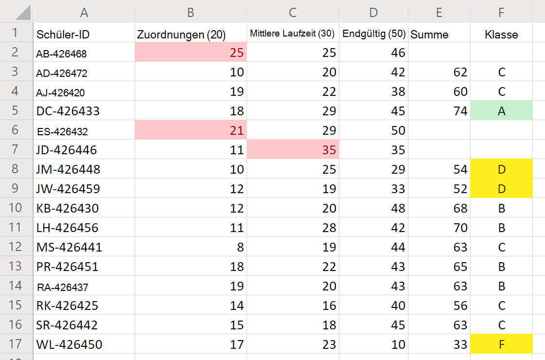
Führen Sie das Skript Notenrechner auf dem einzigen Arbeitsblatt aus. Das Skript summiert die Noten und weist jedem Kursteilnehmer eine Buchstabennote zu. Wenn einzelne Noten mehr Punkte aufweisen, als die Aufgabe oder der Test wert ist, wird die beleidigende Note rot markiert, und die Summe wird nicht berechnet. Außerdem sind alle "A"-Noten grün hervorgehoben, während die Noten "D" und "F" gelb hervorgehoben sind.

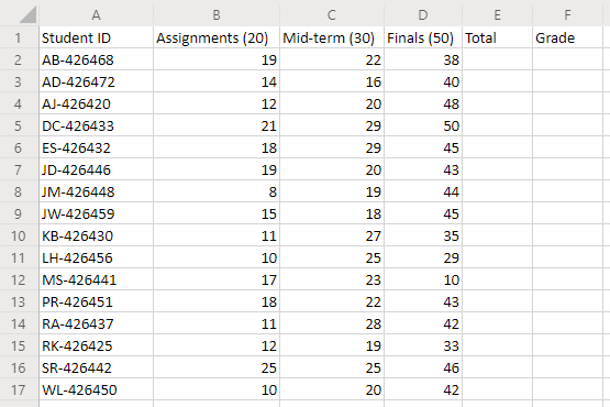
Vor dem Ausführen des Skripts

Nach dem Ausführen des Skripts