Tutorial: Detect and analyze anomalies using KQL machine learning capabilities in Azure Monitor

The Kusto Query Language (KQL) includes machine learning operators, functions and plugins for time series analysis, anomaly detection, forecasting, and root cause analysis. Use these KQL capabilities to perform advanced data analysis in Azure Monitor without the overhead of exporting data to external machine learning tools.

In this tutorial, you learn how to:

• Create a time series
• Identify anomalies in a time series
• Tweak anomaly detection settings to refine results
• Analyze the root cause of anomalies

Note

This tutorial provides links to a Log Analytics demo environment in which you can run the KQL query examples. However, you can implement the same KQL queries and principals in all Azure Monitor tools that use KQL.

Prerequisites

• An Azure account with an active subscription. Create an account for free.
• A workspace with log data.

Permissions required

You must have Microsoft.OperationalInsights/workspaces/query/*/read permissions to the Log Analytics workspaces you query, as provided by the Log Analytics Reader built-in role, for example.

Create a time series

Use the KQL make-series operator to create a time series.

Let's create a time series based on logs in the Usage table, which holds information about how much data each table in a workspace ingests every hour, including billable and non-billable data.

This query uses make-series to chart the total amount of billable data ingested by each table in the workspace every day, over the past 21 days:

Click to run query

let starttime = 21d; // The start date of the time series, counting back from the current date
let endtime = 0d; // The end date of the time series, counting back from the current date
let timeframe = 1d; // How often to sample data
Usage // The table we’re analyzing
| where TimeGenerated between (startofday(ago(starttime))..startofday(ago(endtime))) // Time range for the query, beginning at 12:00 AM of the first day and ending at 12:00 AM of the last day in the time range
| where IsBillable == "true" // Include only billable data in the result set
| make-series ActualUsage=sum(Quantity) default = 0 on TimeGenerated from startofday(ago(starttime)) to startofday(ago(endtime)) step timeframe by DataType // Creates the time series, listed by data type 
| render timechart // Renders results in a timechart

In the resulting chart, you can clearly see some anomalies - for example, in the AzureDiagnostics and SecurityEvent data types:

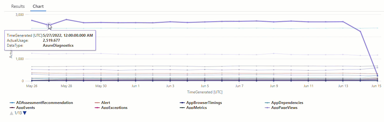
Next, we'll use a KQL function to list all of the anomalies in a time series.

Note

For more information about make-series syntax and usage, see make-series operator.

Find anomalies in a time series

The series_decompose_anomalies() function takes a series of values as input and extracts anomalies.

Let's give the result set of our time series query as input to the series_decompose_anomalies() function:

Click to run query

let starttime = 21d; // Start date for the time series, counting back from the current date
let endtime = 0d; // End date for the time series, counting back from the current date
let timeframe = 1d; // How often to sample data
Usage // The table we’re analyzing
| where TimeGenerated between (startofday(ago(starttime))..startofday(ago(endtime))) // Time range for the query, beginning at 12:00 AM of the first day and ending at 12:00 AM of the last day in the time range
| where IsBillable == "true" // Includes only billable data in the result set
| make-series ActualUsage=sum(Quantity) default = 0 on TimeGenerated from startofday(ago(starttime)) to startofday(ago(endtime)) step timeframe by DataType // Creates the time series, listed by data type
| extend(Anomalies, AnomalyScore, ExpectedUsage) = series_decompose_anomalies(ActualUsage) // Scores and extracts anomalies based on the output of make-series 
| mv-expand ActualUsage to typeof(double), TimeGenerated to typeof(datetime), Anomalies to typeof(double),AnomalyScore to typeof(double), ExpectedUsage to typeof(long) // Expands the array created by series_decompose_anomalies()
| where Anomalies != 0  // Returns all positive and negative deviations from expected usage
| project TimeGenerated,ActualUsage,ExpectedUsage,AnomalyScore,Anomalies,DataType // Defines which columns to return 
| sort by abs(AnomalyScore) desc // Sorts results by anomaly score in descending ordering

This query returns all usage anomalies for all tables in the last three weeks:

Looking at the query results, you can see that the function:

• Calculates an expected daily usage for each table.
• Compares actual daily usage to expected usage.
• Assigns an anomaly score to each data point, indicating the extent of the deviation of actual usage from expected usage.
• Identifies positive (1) and negative (-1) anomalies in each table.

Note

For more information about series_decompose_anomalies() syntax and usage, see series_decompose_anomalies().

Tweak anomaly detection settings to refine results

It's good practice to review initial query results and make tweaks to the query, if necessary. Outliers in input data can affect the function's learning, and you might need to adjust the function's anomaly detection settings to get more accurate results.

Filter the results of the series_decompose_anomalies() query for anomalies in the AzureDiagnostics data type:

The results show two anomalies on June 14 and June 15. Compare these results with the chart from our first make-series query, where you can see other anomalies on May 27 and 28:

The difference in results occurs because the series_decompose_anomalies() function scores anomalies relative to the expected usage value, which the function calculates based on the full range of values in the input series.

To get more refined results from the function, exclude the usage on the June 15 - which is an outlier compared to the other values in the series - from the function's learning process.

The syntax of the series_decompose_anomalies() function is:

series_decompose_anomalies (Series[Threshold,Seasonality,Trend,Test_points,AD_method,Seasonality_threshold])

Test_points specifies the number of points at the end of the series to exclude from the learning (regression) process.

To exclude the last data point, set Test_points to 1:

Click to run query

let starttime = 21d; // Start date for the time series, counting back from the current date
let endtime = 0d; // End date for the time series, counting back from the current date
let timeframe = 1d; // How often to sample data
Usage // The table we’re analyzing
| where TimeGenerated between (startofday(ago(starttime))..startofday(ago(endtime))) // Time range for the query, beginning at 12:00 AM of the first day and ending at 12:00 AM of the last day in the time range
| where IsBillable == "true" // Includes only billable data in the result set
| make-series ActualUsage=sum(Quantity) default = 0 on TimeGenerated from startofday(ago(starttime)) to startofday(ago(endtime)) step timeframe by DataType // Creates the time series, listed by data type
| extend(Anomalies, AnomalyScore, ExpectedUsage) = series_decompose_anomalies(ActualUsage,1.5,-1,'avg',1) // Scores and extracts anomalies based on the output of make-series, excluding the last value in the series - the Threshold, Seasonality, and Trend input values are the default values for the function 
| mv-expand ActualUsage to typeof(double), TimeGenerated to typeof(datetime), Anomalies to typeof(double),AnomalyScore to typeof(double), ExpectedUsage to typeof(long) // Expands the array created by series_decompose_anomalies()
| where Anomalies != 0  // Returns all positive and negative deviations from expected usage
| project TimeGenerated,ActualUsage,ExpectedUsage,AnomalyScore,Anomalies,DataType // Defines which columns to return 
| sort by abs(AnomalyScore) desc // Sorts results by anomaly score in descending ordering

Filter the results for the AzureDiagnostics data type:

All of the anomalies in the chart from our first make-series query now appear in the result set.

Analyze the root cause of anomalies

Comparing expected values to anomalous values helps you understand the cause of the differences between the two sets.

The KQL diffpatterns() plugin compares two data sets of the same structure and finds patterns that characterize differences between the two data sets.

This query compares AzureDiagnostics usage on June 15, the extreme outlier in our example, with the table usage on other days:

Click to run query

let starttime = 21d; // Start date for the time series, counting back from the current date
let endtime = 0d; // End date for the time series, counting back from the current date
let anomalyDate = datetime_add('day',-1, make_datetime(startofday(ago(endtime)))); // Start of day of the anomaly date, which is the last full day in the time range in our example (you can replace this with a specific hard-coded anomaly date)
AzureDiagnostics	
| extend AnomalyDate = iff(startofday(TimeGenerated) == anomalyDate, "AnomalyDate", "OtherDates") // Adds calculated column called AnomalyDate, which splits the result set into two data sets – AnomalyDate and OtherDates
| where TimeGenerated between (startofday(ago(starttime))..startofday(ago(endtime))) // Defines the time range for the query
| project AnomalyDate, Resource // Defines which columns to return
| evaluate diffpatterns(AnomalyDate, "OtherDates", "AnomalyDate") // Compares usage on the anomaly date with the regular usage pattern

The query identifies each entry in the table as occurring on AnomalyDate (June 15) or OtherDates. The diffpatterns() plugin then splits these data sets - called A (OtherDates in our example) and B (AnomalyDate in our example) - and returns a few patterns that contribute to the differences in the two sets:

Looking at the query results, you can see the following differences:

• There are 24,892,147 instances of ingestion from the CH1-GEARAMAAKS resource on all other days in the query time range, and no ingestion of data from this resource on June 15. Data from the CH1-GEARAMAAKS resource accounts for 73.36% of the total ingestion on other days in the query time range and 0% of the total ingestion on June 15.
• There are 2,168,448 instances of ingestion from the NSG-TESTSQLMI519 resource on all other days in the query time range, and 110,544 instances of ingestion from this resource on June 15. Data from the NSG-TESTSQLMI519 resource accounts for 6.39% of the total ingestion on other days in the query time range and 25.61% of ingestion on June 15.

Notice that, on average, there are 108,422 instances of ingestion from the NSG-TESTSQLMI519 resource during the 20 days that make up the other days period (divide 2,168,448 by 20). Therefore, the ingestion from the NSG-TESTSQLMI519 resource on June 15 isn't significantly different from the ingestion from this resource on other days. However, because there's no ingestion from CH1-GEARAMAAKS on June 15, the ingestion from NSG-TESTSQLMI519 makes up a significantly greater percentage of the total ingestion on the anomaly date as compared to other days.

The PercentDiffAB column shows the absolute percentage point difference between A and B (|PercentA - PercentB|), which is the main measure of the difference between the two sets. By default, the diffpatterns() plugin returns difference of over 5% between the two data sets, but you can tweak this threshold. For example, to return only differences of 20% or more between the two data sets, you can set | evaluate diffpatterns(AnomalyDate, "OtherDates", "AnomalyDate", "~", 0.20) in the query above. The query now returns only one result:

Note

For more information about diffpatterns() syntax and usage, see diff patterns plugin.

Next steps

Learn more about:

• Log queries in Azure Monitor.
• How to use Kusto queries.
• Analyze logs in Azure Monitor with KQL