Using Azure Machine Learning Notebooks for Quality Control of Automated Predictive Pipelines
By Sander Timmer, PhD, Data Scientist
When building an automated predictive pipeline to have periodically batch-wise score new data there is a need to control for quality of the predictions. The Azure Data Factory (ADF) pipeline will help you ensure that your whole data set gets scored. However, this is not taking into consideration that data can change over time. For example, when prediction churn changes in your website or service offerings could change customer behavior in such a way that retraining of the original model is needed. In this blog post I show how you can use Notebooks in Azure Machine Learning (AML) to get a more systematic view on the (predictive) performance of your automated predictive pipelines.
Define a score quality metric
There is no such thing as a generic way of evaluating your Machine Learning models. Depending on your business needs different demands are set on when predictions are good enough. A good way of looking at real world prediction performance is through cost sensitive learning. Simply said, each error has a different cost in the real world. The University of Nebraska-Lincoln wiki has some great introductory information on this topic. They give also provide the following real world example to put things in perspective: rejecting a valid credit card transaction may cause an inconvenience while approving a large fraudulent transaction may have very negative consequences. In essence, you want to minimize the costs of misclassification.
In this simple example, as we don't know the costs of being wrong, we just want to ensure that 90% of our predictions are within the 0.1 probability score (I call these high confidence predictions). We also want to check for which prediction label our model has more certainty in predicting. This could help in the future to re-train if the cost of error is getting too high for that particular class.
Setting up your Azure Machine Learning experiment
To get our Notebook to always work with the latest scored dataset we have to make some small adjustments to our scoring experiment. For this blog post I edited the Binary Classification: Customer relationship prediction experiment from the Cortana Analytics Gallery. Obviously, you could as easy use any other shared experiment or your own experiment. However, to keep things simple, I decided to just focus on a binary classification problem with not too much data.
I loaded the experiment from the gallery and made a small adjustment to get my scored data being stored in Azure. I did this by introducing a new writer module, after a Score Model module. In this Writer module we are going to write the scored dataset to Azure Blob Storage. Make sure you change the default behavior to overwrite, otherwise the second time this experiment runs it will fail. This is the only change I made in this experiment, thus after it has run once and a CSV file has been created you can close the experiment.
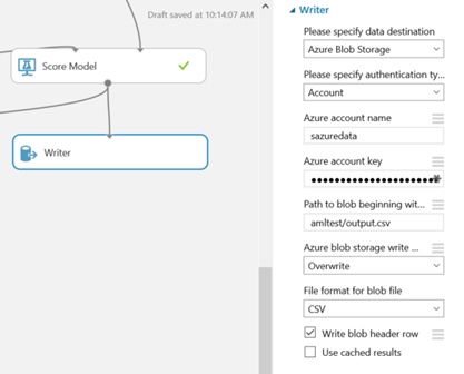
Obviously, if your automated predictive pipeline is using CSV files in blob containers you could skip the step above and use that blob container instead.
Reading and writing files into Azure Machine Learning Notebooks
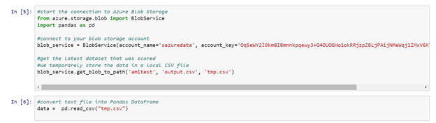
One of the useful features of having Notebook in running in the cloud is that they offer an easy way to do simple compute on files living in the cloud without having to spin up an VM or download things to your local machine. You can write simple text parsing functionality in Python that can run directly on top of your blob storage containers. See some example code here that I used to quickly parse 1000s of files to only keep those lines I was interested in. For this post we will re-use the first part of that post, the reading of the CSV file that is located in the blob storage container. You could re-use the writing part to collect and store rows of data that are of interest for further analyses.
Creating a quality control Python Notebook
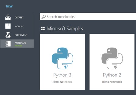
In the AML Studio we can create a new Python 2.x Notebook (Currently there is also support for Python 3.x). We do this by going to New -> Notebooks -> Blank Python 2 Notebook.
First thing I need to do this time is converting our plain text file (which we know is a CSV file) into something more useful. In this example I convert the CSV file into a Pandas DataFrame using the following code:
Note of warning when using Notebook, printing large amounts of rows will make your browser crash, hence, use .head(n=10) on your Pandas DataFrames to get a quick glance of what is inside your DataFrame might help.
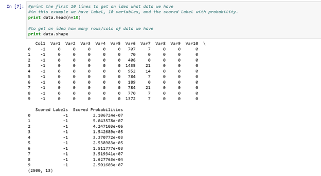
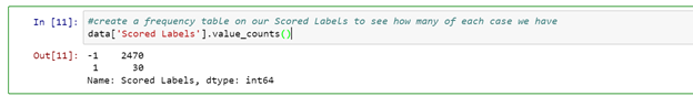
Now I have the data inside our Notebook we can play around and have a look how well our predictions are. First we check how many of each Scored Label I have predicted in our current dataset. For my sample dataset I have 2470 with a Scores Label -1 and 30 in Scored Label 1.
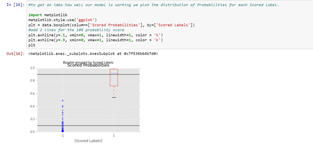
I then had a look at the distribution of the Scored Probabilities for each of the Scored Labels. To do this, I have created boxplots using Matplotlib for each independent Scored Label. I also included 2 lines showing the 0.10 Scored Probability threshold. As can be seen, for the -1 Scored Labels most have a very low Scored Probability. This means that our model is very certain for the prediction of this type in most cases.
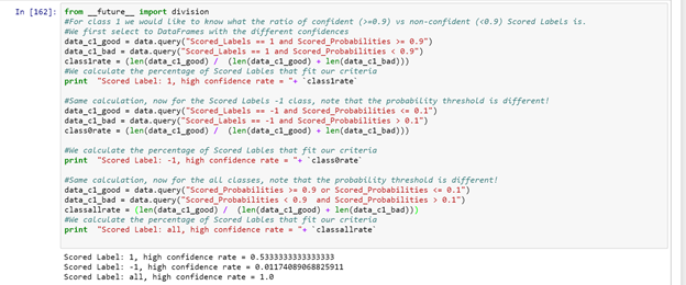
As we decided in the beginning, for this example we are just interested to see how confident our model is and if it is able to predict 90% of the cases with a 0.1 confidence interval. To calculate this, I use the query interface for Pandas DataFrames. In the query interface you can write SQL like on your DataFrames, making data comparison/slicing/indexing extremely straightforward. I decided to determine the quality of prediction per class and overall with the code below. As can be seen, on overall we score 98% with a high confidence. However, when looking at each individual Scored Label there is a high discrepancy between both labels. This means that it might be wise to re-train the model in the near future when enough data is collected for the 1 class.
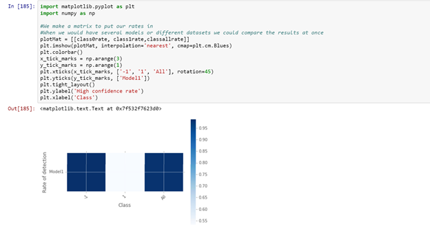
Now we got this in numerical ways, I also decided to make a simple matrix plot, showing the performance of the model, measured by the ratio of confident scores. The code is easy adjustable that if you would have multiple models that you score batch-wise you could compare them visually and decide which models has highest confidence for the given dataset.
Next steps
While the Notebook built for this post will help you understand the performance of your models when taken into production there are still many options for improvement. For example, when using ADF to batch-wise score new data you could label the scored data in such a way you can study the model performance between batches. This way, it could become clear that there is some model performance fluctuation that could be attributed to an external event. For example, weather or holidays could make your model underperform and only by comparing performance over time this could become obvious.
Another potential improvement could be to trigger re-training of the model once performance hits some low criteria for your evaluation metric. In this case you could start collecting all rows of data on which the current model is not confident with its predictions. If enough data has been collected, you could start labelling these data points with the correct label and use this as an addition for your original training data set. This way your model performance will, most likely, improve on the cases that previously were hard to score.