Estimating Hidden Bug Count -- Part 2/3
Previous part: introduction and simpler theory
Next: Flowchart Summary and Limitations
Part 3: Harsh Reality
That simple logic is nice, but practice makes it questionable for at least two reasons:
- Bugs found by either of the parties are fixed. After that, another party gets no chances to find them again.
- Product development results in code changes and new code introductions, further obscuring the picture.
The good news is that in “classic” software with a clear notion of “version” (such as an operating system or a browser) both effects could be accounted for.
The 2nd one is easier. By shipping version 1.0 of the product to the customer you effectively create a nearly frozen snapshot of it affected only by bug fixes. External Researchers will be testing that version. Of course, Internal Engineering will be working with version 2.0 which is different. But it is usually quite easy to filter their discoveries (for analytical purposes) down to the codebase common with 1.0. So if we apply the method to the codebase that is shared between 1.0 and 2.0, we can work around the issue #2.
#1 is trickier. Intuitively it's clear that shared bugs can still appear in a changing product if both parties hit the same bug while it's active – i.e., between the moments it was found and fixed. But knowing the quantity of such discoveries requires more precise tracking of bug counts at each intermediate moment of time.
And one of the ways to achieve that is to describe bug populations with a system of differential equations.
The next few pages treat that subject. If you are not interested, just jump directly to the Step by Step Guide where the results are applied.
Bug Population Dynamics: General Case
Let’s introduce the following variables:
- E is the count of externally found active (i.e., not fixed yet) bugs that are not Shared bugs (so they are reported only once and by external sources only)
- I isthe count of internally found active non-shared bugs
- S is the count of active shared bugs, found by both internal and external entities. That does not include internal Duplicate bugs where the same bug is seen by two or more internal entities.
- B is the total bug count in the system (obviously we are talking about some fixed class of them, e.g., memory corruptions)
Each of them is a function of observation time t passed since version 1.0 of the product was released.
We will assume that bugs are found and fixed with rates linearly proportional to their amount. While that is obviously a simplification, it is probably somewhat close to the reality, since when bug counts increase more developer resources are poured in to fix them.
That will bring along a few more variables:
- x is the rate of external bugs search and reporting per small unit of time (e.g., one month), relative to the total number of bugs. For instance, if x = 0.1 that mean Externals can find 10% of the bugs in a product in one month.
- y is bugs discovery rate for internal engineering, defined in the same manner as x.
- f is the rate of internal bug fixing relative to the total count of active bugs, per unit of time [i.e., f = -(dA/dt)/A, where A is the count of the active bugs].
Strictly speaking, none of these variables are constants. They change over time and as bug counts change. But we need to start somewhere, so let's use that model as a first order approximation.
We will also assume that f is the same for all bugs regardless of whether they are internal or external. The case of significant difference could be reduced to the solution of uniform f, as will be shown later.
In these variables, the dynamics of each bug category is described by the following system of differential equations:
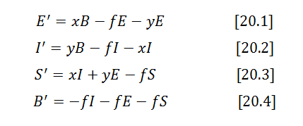
The first line says that active External bugs E are found with frequency x per year proportionally to the total bugs count B in the system, and are fixed with frequency f proportionally to their amount E, and sometimes also move away from External to Shared category when Internals find them, which happens with frequency y.
The 2nd equation is the same but with respect to the Internal active bugs count I.
The 3rd says that active Shared bugs are created when one party hits another's existing active bugs, and destroyed by fixing with a common fix rate f. We assume here that internal sources don't have knowledge of external bugs to check for duplicates before filing. That's not exactly the case but is likely close to reality; if needed, a modification to account for that effect is relatively easy.
Finally, the 4th equation describes the overall bug population, and states simply that the total bug count in the product is reduced when active bugs are fixed.
There is really nothing of a rocket science behind solving that system, but it takes a few pages if done by hand on paper, so I’ll spare you from that and will just write down the answer that shows how each bug category behaves over time:

where
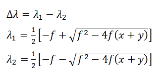
And B0 is the total initial bug count in the system.
Hmm?…
This is ugly.
Extracting B0 from that system is technically possible. You "just" fit those curves to the observed bug rates… in theory… and obtain miserable nonsense in practice because of the data noise, model imperfections, and unmanageable complexity.
Fortunately, we don’t need full precision here. In real life we often deal only with special cases – such as very short or very long observation times, or very high fix frequency, and so on. And it turns out that in this case it is possible to effectively “tile” most practically useful situations with those simpler special cases.
So let’s derive them from the general form.
Case A. Short Observation Times
At very short observation durations, such that t << 1/f and t << 1/(x+y), functions [30] – [60] could be expanded into low-order time series, and then it is possible to show that:
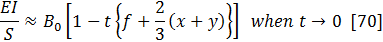
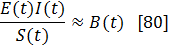
Since nobody prevents us from declaring t = 0 at any arbitrary moment of product lifetime, this means a simple and very powerful thing: as long as there are statistically enough active bugs of Internal, External, and Shared category opened far less than 1/f time ago, the total bug count in the system can be estimated at the current moment of time as simply as:

This works regardless of the frequency of product fixes and (as will be shown later) even if there is an asymmetry between fix rates for internal and external bugs.
Case B. Long Observation Times
At very long observation times such that t >> 1/f and t >> 1/(x+y) most of the bugs found are fixed, so there are very few (if any at all) of them in the active state suitable for use in expression [80].
However, fixed bugs of each category will probably be numerous. Can we use their counts instead?
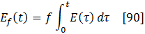
Let’s call them Ef, If, and Sf -- similarly to the corresponding active categories (index “f” stands for “fixed”). Each of those is obtained by integrating the corresponding active bug fixes over time, e.g.:
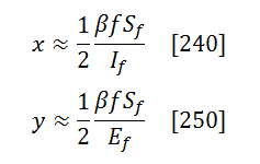
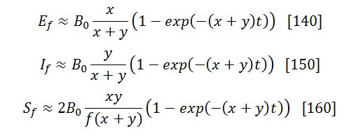
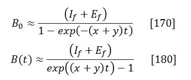
Using these variables and simplifying the full solution for the case of t -> ∞ , one can show that
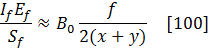
where
[And estimates for x and y could be used to verify if indeed t >> 1/(x+y)]
The relation between the current bug count B(t) and the initial one B0 is:

Case C. Sufficiently High Fix Rate
When f >> (x+y) another useful simplification arises for times such that t >> 1/f:
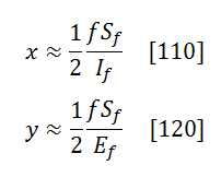
And then
with x and y provided by [110] and [120].
This set of simplifications actually covers (mostly) all of the problem space. Indeed:
a) If there is statistically significant number of active bugs in the product, expression [80] approximately solves the problem, since we can declare t = 0 at any moment of time.
b) If not, but there is statistically significant number of fixed/closed bugs in the product that means the observation time is far greater than typical fix time. In other words, we are in the t >> 1/f domain. Since most bugs are in the fixed rather than active state that also means f >> (x+y) and expressions [170] and [180] provide the answer.
e) In other cases there are either not enough bugs to make a call, or we are in the "narrow" intermediate time window of t ≈ 1/f. We should either wait, or use the full solution [30]-[60].
Case D. Asymmetric Fix Rate
Situations when fix rates for internal and external bugs are significantly different are conceivable. How would our logic work for them?
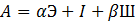
Let f be the fix rate of internal bugs, αf – fix rate of external bugs, and βf – of shared bugs. System [20] becomes then:

Technically, it could be solved from scratch, but we can avoid that by making variable substitution:
and introducing an intermediate variable
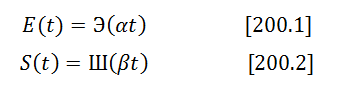
That would result in the solutions of the same form as [30] – [60] with the following input variable replacements:
For E(t): t -> αt, x-> x/α , y->y/α [210]
For S(t): t -> β t, x-> x/β , y->y/β [220]
The short-term estimate then is exactly the same as [80] (i.e., not sensitive to the asymmetry):
Long-term is more difficult because sufficiently high fix rate discrepancy may cause a situation where ft << 1 while α*ft >> 1 at the same time. Technically, the answer would need to be derived from full case [30]-[60], but there is one potential alternative here.
That is to consider internal product version as the primary target, with f being the frequency of internal fixes, and E meaning not all externally reported bugs but only those that affect the internal product version currently in development. If fix rate discrepancy is smaller for the internal version (which is probably more reasonable to expect), long-term estimates [170]-[180] may still be applicable within that interpretation, provided the following changes in variables interpretations:
- f is the frequency of internal fixes for bugs of internal origin
- E is the count of those externally reported bugs that affect the internal product version currently in development
- B is the count of those bugs in internal (2.0) version that affect external (1.0) version
Also the expressions for x and y in this case change to