Is Pluto a Planet?
Is Pluto a planet?
And how is that question related to Data Science?
For sure, physical properties of Pluto do not change if we call it a "planet", a "dwarf planet", a "candelabrum", or a "sea cow". Pluto stays the same Pluto regardless of all that. For physics or astronomy, naming does not really matter.
Yet we don't expect to find publications on Pluto in the Journal of Marine Biology. They belong to astronomy or planetary science. So, for information storage and retrieval naming does matter, and does a lot.
From that standpoint, the distinction is material. When we study "real" planets like Mars or Venus we often mention features that only "real" planets tend to have -- such as atmospheres, tectonic activity, or differentiated internal structure. Small asteroids and "boulders" rarely if ever have any of that. Reflecting those physical differences, the vocabularies would likely be different as well.
Thus, we may classify something as a "planet" if language used with respect to that object follows the same patterns as language used with "real" planets. Simply because it would be easier to store, search and use the information when it's organized that way.
But is that difference detectable? And if yes, is it consistent?
That calls out for an experiment:
- Collect a body of texts concerning an object that we confidently consider a planet -- say, Mars.
- Collect a body of texts (preferably from the same source) associated with "definitely not a planet" -- say, a comet or an asteroid.
- Do the same for Pluto.
- Using text mining algorithms, compute vocabulary similarity between each pair of subjects and check whether Pluto's texts language better resembles that of Mars -- or of a non-planetary object.
I ran that experiment. The results suggest that Pluto indeed is a planet with respect to how we talk about it. The details are provided below.
Algorithm Outline
Assuming the documents are represented as a collection of .txt files, for each planetary body:
- Read all text from the files.
- Split it into tokens using a set of splitters like ' ' (whitespace), '.' (dot) or '-' (dash) (42 in total, see the code for the full list).
- Drop empty tokens.
- Drop tokens that are too short. In these experiments, 2 was the threshold, but I saw virtually the same results with 1 or 3.
- Drop tokens consisting only of digits (e.g., "12345")
- Drop the so-called "stop words", which are very common tokens like "a" or "the" that rarely carry any significant information. I used the list from Wikipedia, extended with a few terms like "fig" (a short for "figure"), or "et" and "al" common in scientific context.
- Run Porter suffix stemming algorithm on each token. The algorithm maps grammatical variations of the same word into common root (e.g., "read", "reads", "reading" -> "read"). Published in 1980, the algorithm is still considered a "golden standard" of suffix stemming, not least because of its high performance. While the algorithm description is clear and relatively straightforward, the implementation is very sensitive to getting all the details exactly right. So I used publicly available C# implementation by Brad Patton from Martin Porter's page (greatest thanks to the author!)
- Again drop tokens that were too short, if any at this point.
- Add the resulting keywords to the collection of words counts. Thus, if A is such a collection, then A[a] is be the count of word a in A.
- While performing steps 1-9 above, also maintain a count of documents that use each word. This is done to be able to give less common words that carry more information (e.g., "exosphere" vs. "small") more impact on documents similarity comparison, via assigning them the so called "tf-idf" weight. After a few experiments, I arrived to the following definition of IDF weight per word:
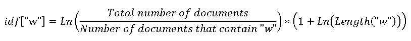
- While the extra length term deviates from more
- traditional definitions
- , I found the discriminative power of this approach to be better than several other variations tested.
- Using the formula above, also compute and store the idf[a] collection for all words in the corpus.
When these collections (A[a] and idf[a]) are produced for each topic (i.e., one pair for Mars, another for Pluto), compute corpus pairwise cosine similarities:
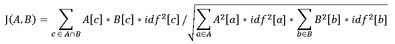
[Again, several other variations were tested, with this one producing the best classes discrimination in tests]
The resulting metric, J(A,B), is the vocabulary similarity between the sets of documents A and B, ranging from 0 (totally different) to 1 (exactly the same).
The code is here if you want to examine it, except for the Porter algorithm which as I mentioned was adopted verbatim from C# implementation by Brad Patton.
OK. The code is written. How do we know it really works? That's what testing is for.
Test 1. Classical Music vs. Chemistry
For this test, two bodies of text were chosen.
The first consisted of Wikipedia articles on inert gases Helium, Neon, Argon, Krypton and Xenon, sections starting after the table of content, and continuing (but not containing) to "References" or "See Also". The second corpus consisted of articles on classical music composers Bach, Beethoven, Mozart and Rachmaninoff, similarly pre-filtered.
Two test subjects were Wikipedia article about Oxygen (gas), and Wikipedia article about Oxygene, a famous musical album of Jean Michelle Jarre, the composer. The question was: can this code properly attribute those test articles as belonging to gases or music?
After fixing couple of bugs, some fine-tuning and experimentation, the code kicked in and produced the following output:
| Gases | Composers | Oxygen (gas) | Oxygene (album) | |
| Gases | 100% (0.237) | 2.33% (0.092) | 23.3% (0.197) | 1.38% (0.244) |
| Composers | 2.33% (0.092) | 100% (0.225) | 3.61% (0.152) | 5.74% (0.348) |
| Oxygen (gas) | 23.3% (0.197) | 3.61% (0.152) | 100% (0.347) | 2.25% (0.189) |
| Oxygene (album) | 1.38% (0.244) | 5.74% (0.348) | 2.25% (0.189) | 100% (0.587) |
The percentage is the degree of similarity J(A, B). The number in parenthesis is the support metric of how many unique words entered the intersection set, relative to word count of the smaller set. Highlighted is the largest similarity (except to self) in each row. As you can see, the method correctly attributed Oxygen (gas) to gases, and Oxygen (musical album) to Music/Composers.
And yes, I'm explicitly computing the distance matrix twice -- from A to B and from B to A. That is done on purpose as an additional built-in test for implementation correctness.
OK, this was pretty simple. Music and chemistry are very different. Can we try it with subjects somewhat closer related?
Test 2. Different Types of Celestial Bodies, from Wikipedia again
Now we will use seven articles, with all the text up to "References" or "See also" sections:
- Sirius and Betelgeuse (both are stars)
- Mars and Venus (both are "first class" citizens in the world of planets)
- Comet 67P/Churyumov–Gerasimenko and Halley's Comet (both are comets, definitely not planets)
- Pluto (why not give it a try?)
The resulting similarity matrix:
| 67P | Betelgeuse | Halley Comet | Mars | Pluto | Sirius | Venus | |
| 67P | 100% (0.481) | 0.76% (0.259) | 2.8% (0.23) | 1.78% (0.286) | 0.696% (0.234) | 0.297% (0.202) | 1.13% (0.252) |
| Betelgeuse | 0.76% (0.259) | 100% (0.307) | 1.27% (0.183) | 2.66% (0.133) | 1.66% (0.159) | 6.9% (0.204) | 2.86% (0.167) |
| Halley Comet | 2.8% (0.23) | 1.27% (0.183) | 100% (0.393) | 2.05% (0.195) | 2.12% (0.159) | 1.48% (0.15) | 1.97% (0.164) |
| Mars | 1.78% (0.286) | 2.66% (0.133) | 2.05% (0.195) | 100% (0.289) | 3.87% (0.175) | 1.76% (0.19) | 9.11% (0.191) |
| Pluto | 0.696% (0.234) | 1.66% (0.159) | 2.12% (0.159) | 3.87% (0.175) | 100% (0.326) | 1.07% (0.155) | 2.68% (0.15) |
| Sirius | 0.297% (0.202) | 6.9% (0.204) | 1.48% (0.15) | 1.76% (0.19) | 1.07% (0.155) | 100% (0.448) | 2.01% (0.171) |
| Venus | 1.13% (0.252) | 2.86% (0.167) | 1.97% (0.164) | 9.11% (0.191) | 2.68% (0.15) | 2.01% (0.171) | 100% (0.334) |
What do we see? Stars are correctly matched against stars. Comets -- against comets (although not very strongly). "True" planets are matched to "true" planets with much greater confidence. And Pluto? Seems like the closest match among the given choices is... Mars. With the next being... Venus!
So at least Wikipedia, when discussing Pluto, uses more "planet-like" language rather than "comet-like" or "star-like".
To be scientifically honest -- if I add Ceres to that set, the method correctly groups it with Pluto, sensing the "dwarfness" in both. But the next classification choice for each is still strongly a "real" planet rather than anything else. So at least from the standpoint of this classifier, a "dwarf planet" is a tight subset of a "planet" rather than anything else.
Now let's put it to real life.
Test 3. Scientific Articles The 47th Lunar and Planetary Science Conference held in March 2016 featured over two thousand great talks and poster presentations on the most recent discoveries about many bodies of the Solar System, including Mars, Pluto, and 67P/Churyumov–Gerasimenko comet. The program and abstracts of the conference are available here. What if we use them for a test?
This was more difficult than it seems. For ethical reasons, I did not want to scrape the whole site, choosing to use instead a small number (12 per subject) of purely randomly chosen PDF abstracts. Since the document count was low, I decided not to bother with PDF parsing IFilter and to copy relevant texts manually. That turned out to be a painful exercise requiring great attention to detail. I needed to exclude authors lists (to avoid accidentally matching on people or organization names), references, and manually fix random line-breaking hyphens in some documents. For any large-scale text retrieval system, this process would definitely need serious automation to work well.
But finally, the results were produced:
| 67P | Mars | Pluto | |
| 67P | 100% (0.252) | 17.9% (0.126) | 19.7% (0.132) |
| Mars | 17.9% (0.126) | 100% (0.224) | 21% (0.111) |
| Pluto | 19.7% (0.132) | 21% (0.111) | 100% (0.21) |
The differences are far less pronounced, probably because the texts have very similar origins and format restrictions, and use the same highly specialized scientific vocabulary. Still, within the space of this data set, Pluto was slightly more of a planet rather than of a comet!
Closing Remarks
How seriously should these results be taken?
First, they are obtained on a small data set, with a home-grown classifier, and the differences detected are relatively modest. If anybody wants to take a serious Data Science driven stance on this issue, they should use a much, much larger text corpus.
Second, people are still free to call Pluto a "planet", a "dwarf planet", or a "candelabrum" if that suites them -- regardless of these results.
But there are important points that I wanted to make. First, language use may offer another definition of what is more practical to call "a planet". Second, the language differences behind that definition are objective and measurable. And finally, those differences are representative of the physical world.
Thank you for reading,
Eugene V. Bobukh