Bayesian PCA
This blog has been migrated from community.research.microsoft.com
Original date of blog: February 3, 2009
Original blog author: John Guiver
NOTE: This example and the corresponding code are now directly available in the Infer.NET release.
It’s been a couple of months now since we’ve released Infer.NET to the outside world, and a blog is overdue. I hope those of you have downloaded it are enjoying it and have had a chance at least to go through some of the tutorials to see the scope of what we’re providing. In the process of doing this release, one point of discussion has been the question of to what level we should provide and/or support standard black box models. Here I’m talking about the likes of Bayesian factor analysis, Bayesian PCA, HMMs, Bayesian neural nets, and the Bayes point machine. We have been reluctant to provide these as stock models because we have been keen that Infer.NET should be applied in a more customised way than just throwing data at a generic model. The click through model is an excellent example of a thoughtful customised model which tries to capture the behaviour of a user interacting with a page of results returned by a search engine.
That said, it is often useful in the early stages for a user to look at and employ some standard models just to get started. With the release, we have already provided a set of multi-class Bayes point machine examples which can be used for a variety of classification problems. In this blog I will look at Bayesian principal components analysis – see Chris Bishop’s book Pattern Recognition and Machine Learning for example. Most of you will be familiar with standard Principal Component Analysis which is a widely used technique for dimensionality reduction. Given an observation space of dimension D we would like to find a latent space of lower dimension M (the ‘principal space’) which captures most of the data. The mapping from principal space to observation space is via a linear mapping represented by a mixing matrix W. PCA can be formulated in probabilistic way (‘probabilistic PCA’) and this in itself gives many benefits as itemised in Bishop. If in addition we adopt a Bayesian approach to inferring W, we can also determine the optimal value for M using ‘automatic relevance determination’ (ARD).
A fully Bayesian treatment of probabilistic PCA (including ARD) is quite complex and it might take several weeks of work to implement an efficient deterministic inference algorithm. In Infer.NET, defining the model is 20 to 25 lines of code and a few hours’ work.
I am going to plunge straight in and show the factor graph for Bayesian PCA. Factor graphs are a great representation for probabilistic models, and especially useful if you are going to build models in Infer.NET. If you can draw a factor graph, you should be able to code up the model in Infer.NET (subject to the currently available distributions, factors, and message operators).
I’ll jointly explain aspects of the factor graph and Bayesian PC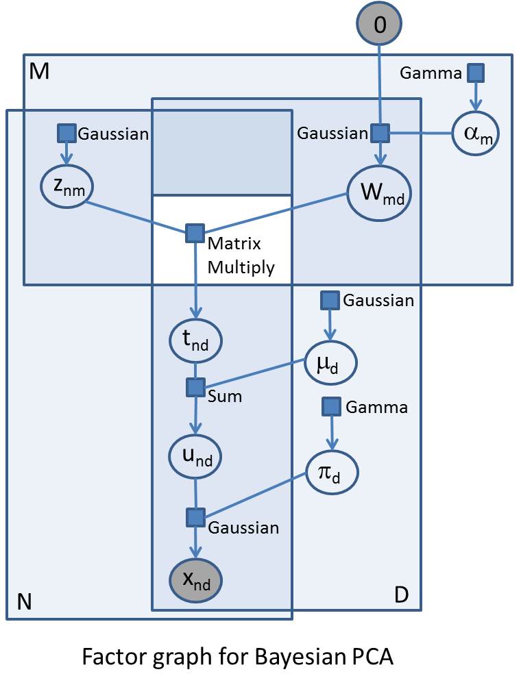 A as I go along. As a reminder, the first thing to note is that the variables in the problem are represented as circles/ovals, and the factors (functions, distributions, or constraints) are represented as squares/rectangles. Each factor is only ever attached to its variables and each variable is only ever attached to its factors. The big enclosing rectangles represent ‘plates’ and show replications of variables and factors across arrays. Factor graphs are important both because they provide a clarifying visualisation of complex probabilistic models and because of the close relationship with the underlying inference and sampling algorithms (particularly those based on local message passing).
The accompanying factor graph shows PCA as a generative model for randomly generating the N observations – these observations can be represented as an NxD array, and so are represented in the factor graph in the intersection of two plates of size N and D respectively. I have explicitly shown all indices in the factor graph to make the comparison with the code clearer. The generative process starts at the top left where, for each observation and for each component in latent space, we sample from a standard Gaussian to give an NxM array Z (with elements znm).
In the top right we have the matrix variable W (elements wmd) which maps latent space to observation space – so this will be an MxD matrix which will post-multiply Z. We have specified a maximum M in advance, but what we really want to do is learn the ‘true’ number of components that explain the data, and we do this by drawing the rows of W from a zero-mean Gaussian whose precisions a (elements a m) we are going to learn. If the precision on a certain row becomes very large (i.e. the variance becomes very small) then the row has negligible effect on the mapping and the effective dimension of the principal space is reduced by the number of such rows. The elements of a are drawn from a common Gamma prior.
The MatrixMultiply factor multiplies the Z with W; as this factor takes two double arrays of variables, it sits outside the plates (shown as a white hole in the surrounding plates). The result of this factor is an NxD matrix variable T (elements tnd). We then add a bias vector variable m (elements m d drawn from a common Gaussian prior) to each row of T to give matrix variable U (elements u*nd*). Finally, the matrix X of observations vector is generated by drawing from Gaussians with mean U and precision given by the vector variable p (elements p d drawn from a common Gamma prior). The elements in this final array of Gaussian factors are the likelihood factors and represent the likelihood of the observations conditional on the parameters of the model. These parameters are W, m and p which we want to infer.
This model is captured in the following few lines of C# code which, as you can hopefully see, directly matches the factor graph (I have omitted the variable and range declarations as these don’t add further insight, but the full code can be found here):
// Mixing matrix
vAlpha = Variable.Array<double>(rM).Named("Alpha");
vW = Variable.Array<double>(rM, rD).Named("W");
vAlpha[rM] = Variable.Random<double, Gamma>(priorAlpha).ForEach(rM);
vW[rM, rD] = Variable.GaussianFromMeanAndPrecision(0, vAlpha[rM]).ForEach(rD);
// Latent variables are drawn from a standard Gaussian
vZ = Variable.Array<double>(rN, rM).Named("Z");
vZ[rN, rM] = Variable.GaussianFromMeanAndPrecision(0.0, 1.0).ForEach(rN, rM);
// Multiply the latent variables with the mixing matrix...
vT = Variable.MatrixMultiply(vZ, vW).Named("T");
// ... add in a bias ...
vMu = Variable.Array<double>(rD).Named("mu");
vMu[rD] = Variable.Random<double, Gaussian>(priorMu).ForEach(rD);
vU = Variable.Array<double>(rN, rD).Named("U");
vU[rN, rD] = vT[rN, rD] + vMu[rD];
// ... and add in some observation noise ...
vPi = Variable.Array<double>(rD).Named("pi");
vPi[rD] = Variable.Random<double, Gamma>(priorPi).ForEach(rD);
// ... to give the likelihood of observing the data
vData[rN, rD] = Variable.GaussianFromMeanAndPrecision(vU[rN, rD], vPi[rD]);
In order to test out this model, I generated 1000 data points from a model with M=3, D= 10. However, when doing inference, I gave it M=6 to see if the inference could correctly determine the number of components. Here is the print-out from a run. As you can see, as expected, only three of the rows of W have significant non-zero entries, and the bias and noise vectors are successfully inferred.
Mean absolute means of rows of W: 0.05 0.24 0.20 0.02 0.21 0.01
True bias: -0.95 0.75 -0.20 0.20 0.30 -0.35 0.65 0.20 0.25 0.40
Inferred bias: -0.90 0.70 -0.22 0.22 0.31 -0.37 0.65 0.17 0.25 0.42
True noise: 1.00 2.00 4.00 2.00 1.00 2.00 3.00 4.00 2.00 1.00
Inferred noise: 0.98 1.99 4.09 2.00 1.08 2.00 2.70 3.51 2.16 1.01
The full C# code for this example can be found here. This code provides a class (BayesianPCA) for constructing a general Bayesian PCA model for which we can specify priors and data at inference time. There is also some example code for running inference and extracting marginals. One important aspect of running inference on this model is that we initially need to break symmetries in the model by initialising the W marginals to random values using the InitialiseTo() method – for another example of this see the Mixture of Gaussians tutorial.
I hope this provides a useful addition to your Infer.NET toolbox and also provides some insight into building models with Infer.NET. Keep the feedback and comments coming.
John Guiver and the Infer.NET team.