A Pricing Engine for Everyone built with AzureML and Python

This post describes the Microsoft Pricing Engine (MPE), a cloud tool for pricing optimization. MPE is easy to integrate into the business process as it uses the business’ transactional history and does not require A/B testing infrastructure to be set up. A double-residual modeling approach in MPE is the newest advanced causal inference approach to mitigating biases inherent in observational studies.

 

Pricing is a core business function for every single company. Yet, there are no one-size-fits-all solutions because every business has a unique history and position in the market. Enormous human, marketing and technical resources are spent on getting pricing right. Today price setting is informed by a combination of experience of long-time employees, competitive market intelligence, experiments and promotions, and supplier forecasts.

Given the abundance of historical data, pricing seems ripe for the application of machine learning. However, the domain is complex, and there are many confounding effects like holidays and promotions. Machine learning tradition prioritizes prediction performance over causal consistency, but pricing decisions need high-quality inference about causation, which is only guaranteed with randomized controlled experiments. Experimentation, also known as A/B testing, is extremely difficult to set up on existing operations systems. Observational approaches are "bolt-on", but tools that guard against the many statistical pitfalls are essential.

In this post, we talk about how to leverage historical data with AzureML and python to build a pricing decision-support application using an advanced observational approach. We call the resulting set of related services the Microsoft Pricing Engine (MPE). We created an Excel-centric workflow interfacing with the services to support interactive use. The demonstration uses the public orange juice data, a popular benchmark dataset in pricing econometrics.

System integrators will be able to use the MPE’s web service interface to build pricing decision support applications on Azure, targeting the mid-size companies with small pricing teams without extensive data science support for customized pricing models.

We will give a bit of theory, discuss how price elasticity is modeled, which potential confounders are included, and the architecture of the pricing engine.

 

A little pricing theory

The core concept is that of price elasticity of demand, a measure of how sensitive the aggregate demand is to price.

Informally, self-price elasticity is the percentage “lift” in sales of a product if we put it on a 1% discount. Most consumer products have elasticities in the range of 1.5-5. Products with more competitors are easier to substitute away from and will have higher elasticity. Discretionary products are more elastic than staples.

 

Lowering the price will improve both sales quantities and hence revenues for products with elasticities e < -1 (negative since the line slopes down). If your product is inelastic (e > -1), you should increase the price – only a little demand will be lost and your revenue will go up.

The above condition holds if you are optimizing only revenue, which is the case if you have negligible marginal cost (e.g. you sell electronic media). More frequently, you have substantial marginal costs, and want to optimize your gross margin (price – marginal cost). Then the constant -1 in the above calculation is replaced by (Price)/(Gross Margin), also known as the inverse Lerner Index. For example, suppose your marginal cost of oranges is $4 and you are selling them for $5. Then you should increase prices at lower elasticities (e > -5), and decrease them otherwise. (This does not account for fixed costs, you may well have complex optimization problem if your marginal costs are already burdened by a share of fixed cost.)

In addition to self-price elasticity, we recognize cross-price elasticity of demand where the demand of a product changes in response to the price of another product. Substitute products have positive cross-elasticity: if price of Tropicana orange juice increases, so do the sales of Minute Maid orange juice, as customers substitute toward Minute Maid. Complementary products have negative cross-elasticities – lowering the price of peanut butter may increase sales for jam even if price of jam stays constant.

The pricing data schema and use case

Input data preparation

Data schemas vary from one data warehouse to another. To get started, our service requires a minimal set of data that every business will likely have:

 

 

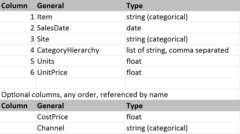
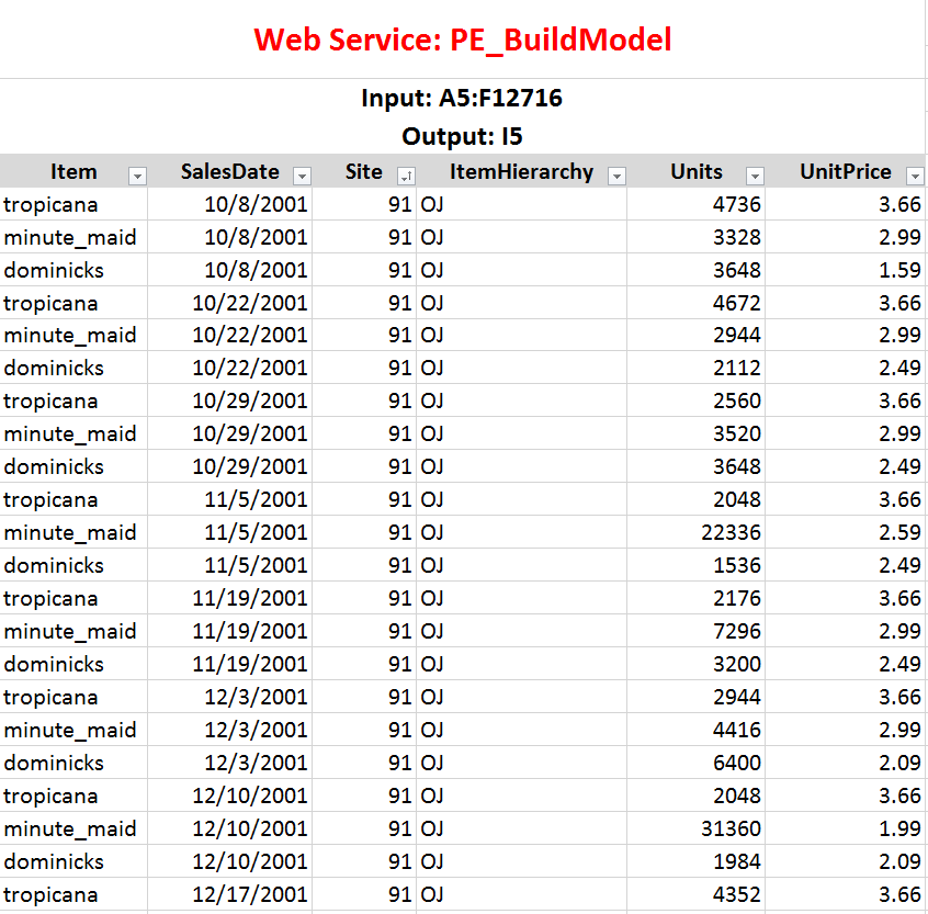
There should be exactly 1 row of data for each Item, Site (and Channel if provided) combination provided. It is best to have at least 2 years’ worth of data so that seasonal effects can be captured. You prepare your data into this format in Excel. For example, if your data is on weekly sales of various brands of orange juice, it would look like this:

 

While we used the Orange Juice dataset, you can use your own data!

Using the pricing services

Let us look at the model building phase, and two analyses that interpret the model. We have made the AzureML web services accessible in Excel using the AzureML Excel plugin. Please contact us if you'd like to receive the pre-configured Excel worksheet.

Building the model and examining elasticities

First, let us estimate the elasticity model from the orange juice data. We gave the data in the columns with gray heading. Then we configured the Pricing Engine Build (PE_Build) service in the AzureML plugin, pointed it to the data and clicked "Predict as Batch" in the AzureML plugin window. This will take about 3 minutes to output the products, locations and date ranges the engine recognizes. We gave our dataset the name OJ_Demo. You can build models from many datasets, just give them different names.

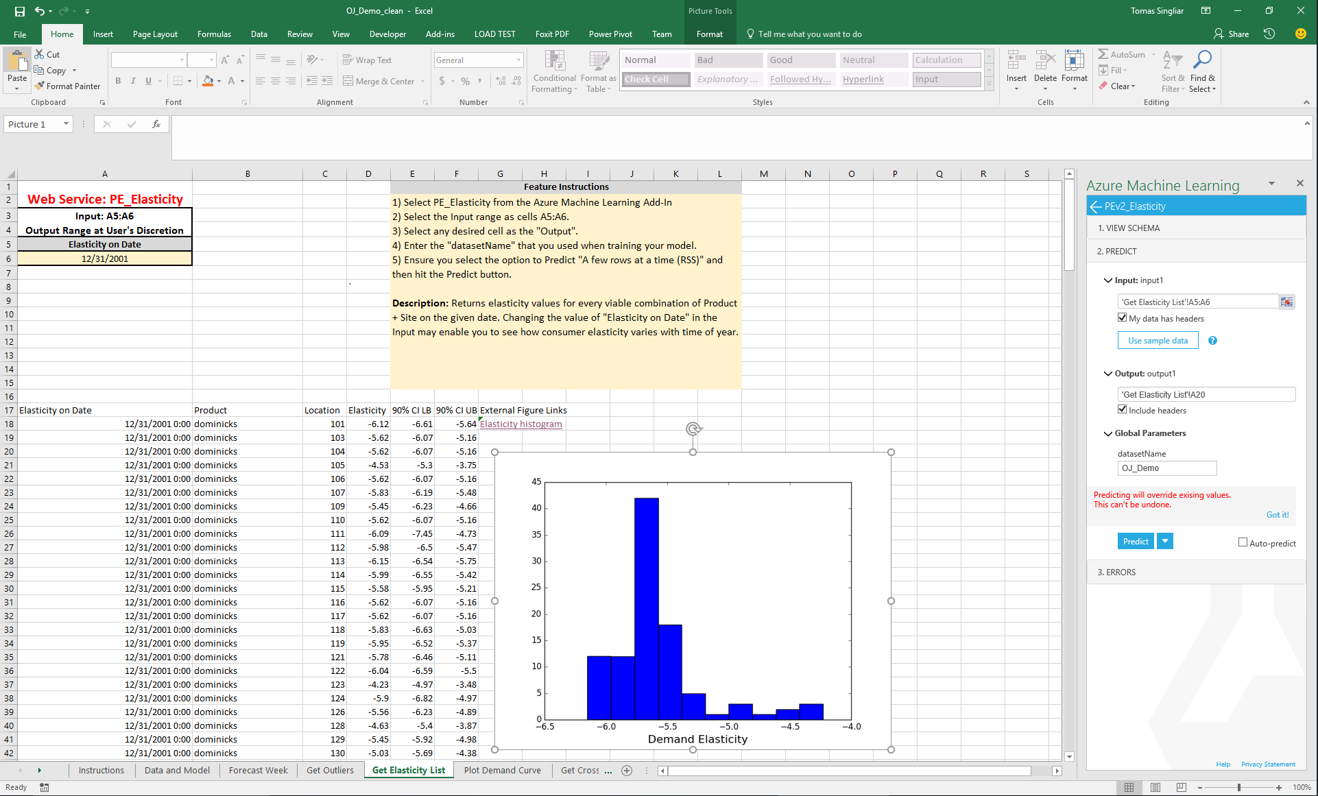
The Elasticity service gives one elasticity per Location (store number) and Product (three brands of OJ). Note we referred to the same dataset "OJ_Demo". We see that the elasticity estimates cluster around -5, which is pretty typical for competitive consumer products, and corresponds to optimal gross margins of approximately 1/5 = 20%. The pricing analyst concludes that any products they are earning less than 20% gross margin are probably underpriced, and vice versa.

 

Interpreting Cross-Elasticities

On the next tab, we consume cross-price elasticities from the PE_CrossPrice.

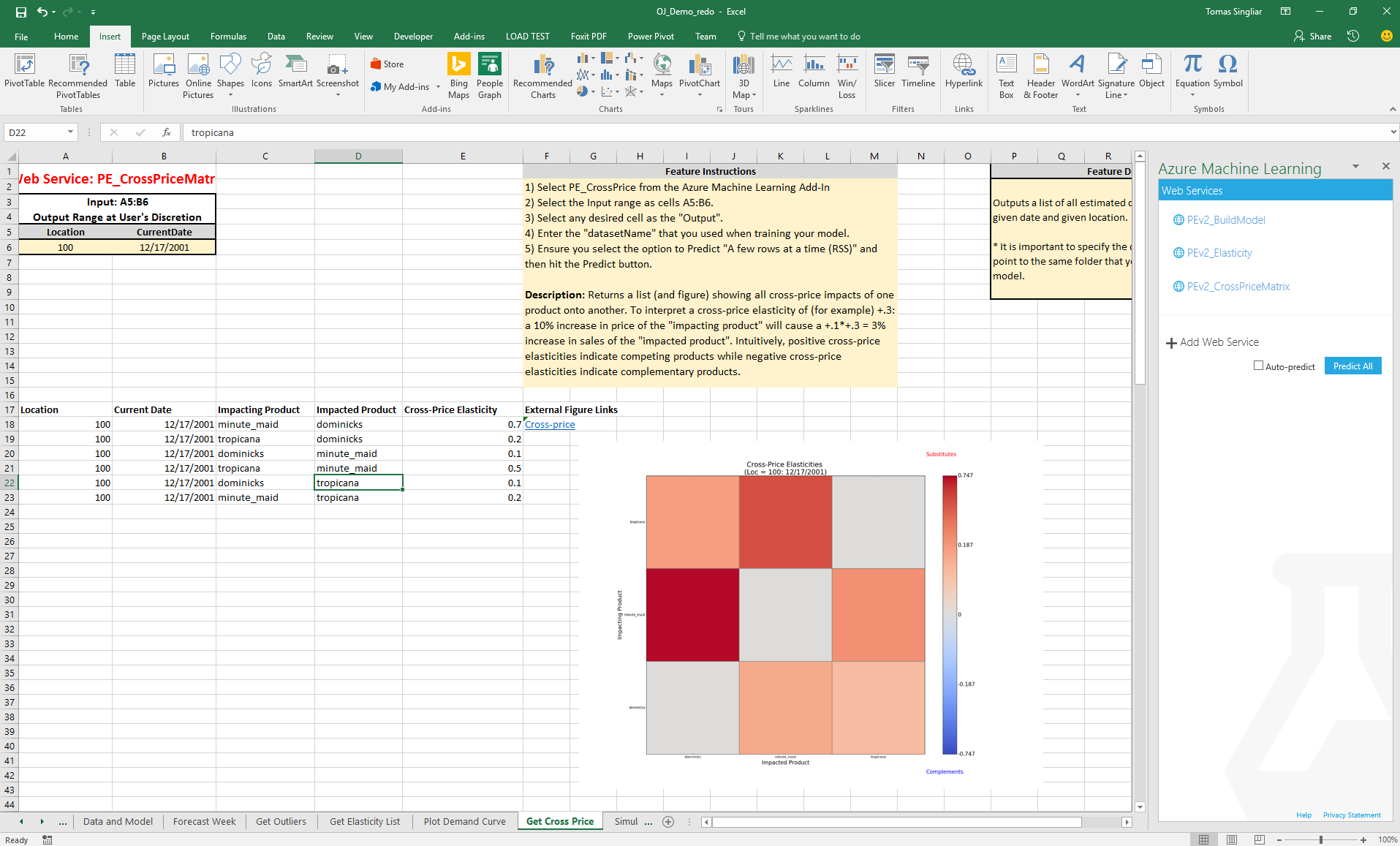
Here, the analysis shows that the products are indeed mostly substitutes - some know this effect as "cannibalization". Note the visualization is not a standard chart, but is a python heat map visualization. This is generated from the engine in the cloud and you get a link to the visual.

Simulating the effect of promotion

Finally, putting it all together, we ask the thousand-dollar question: what happens to our total store sales if we change the price of a brand of OJ? We look at the Promotion Effect tab, which simulates the effect of changing the price of Minute Maid orange juice on the sales of Minute Maid as well as the remaining products. This combines the forecast we have for all products with the estimated self-elasticity of Minute Maid, as well as the cross-price elasticity of Minute Maid and the other two brands in the dataset.

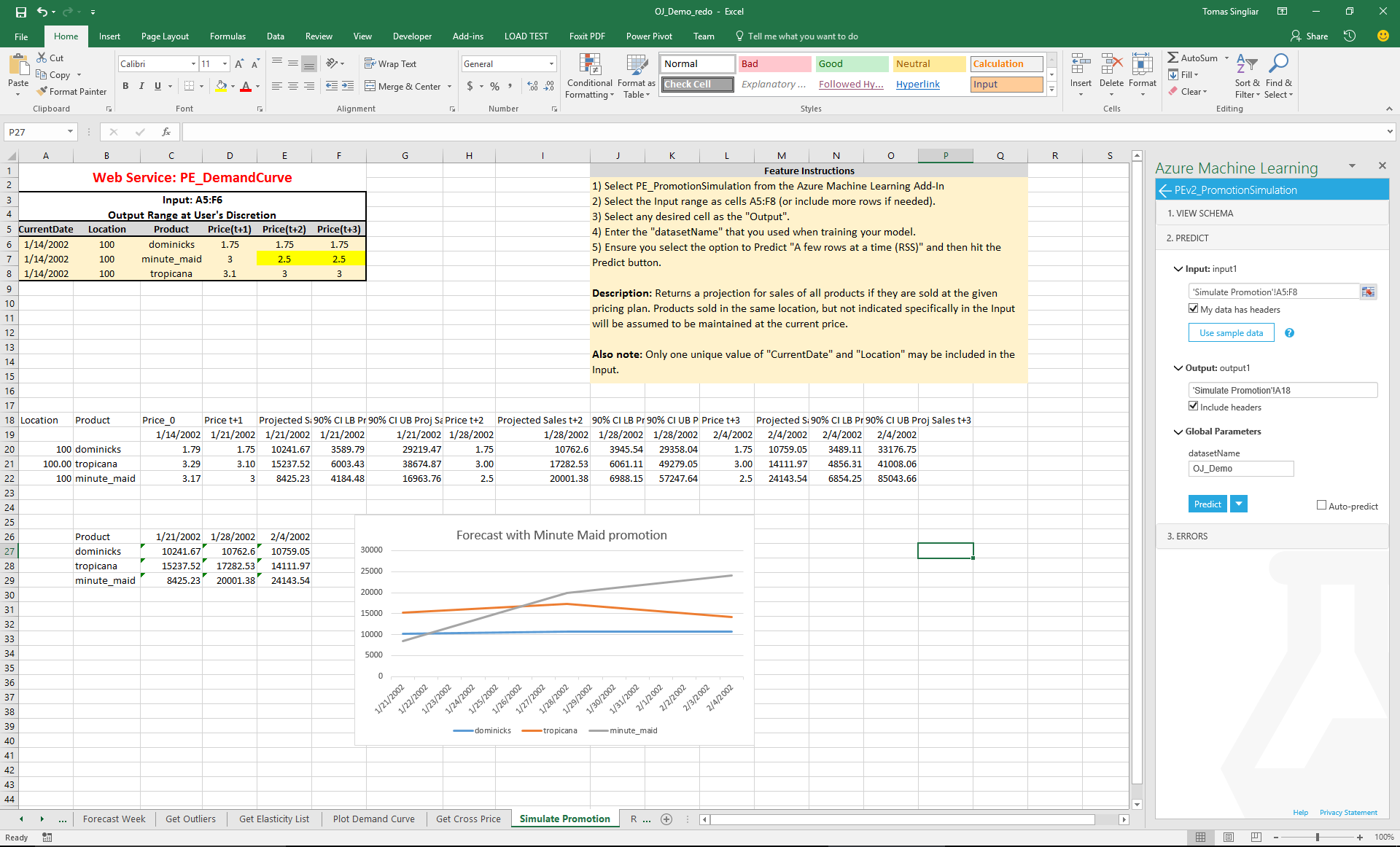
We see that the predicted effects is an increase in demand for Minute Maid, with customers substituting primarily from the other premium brand, Tropicana, while the value brand is mostly unaffected.

The MPE currently offers these services, each corresponding to a tab in the Excel "app":

• Data and Model  (Build the model)
• Elasticity              (Retrieve dataframe and visual of self-elasticities)
• Cross-Elasticity    (Retrieve dataframe and visual of cross-elasticities)
• Forecasts             (Forecasted demands at current, fixed prices)
• Demand Curve    (Forecasted demand at varied prices)
• Promotion Effect (Effect on hypothetical promo on all related products)
• Retrospective      (How good were past forecasts? Confidence bounds.)
• Outliers                (Examine worst forecast misses.)

Pricing engine Azure architecture

The pricing model is implemented in python and wrapped as a web service by AzureML. The figure below shows the Excel-centric workflow backed by the cloud components we use for our simple example. We assume that the data is already exported from a business data source into Excel.

 

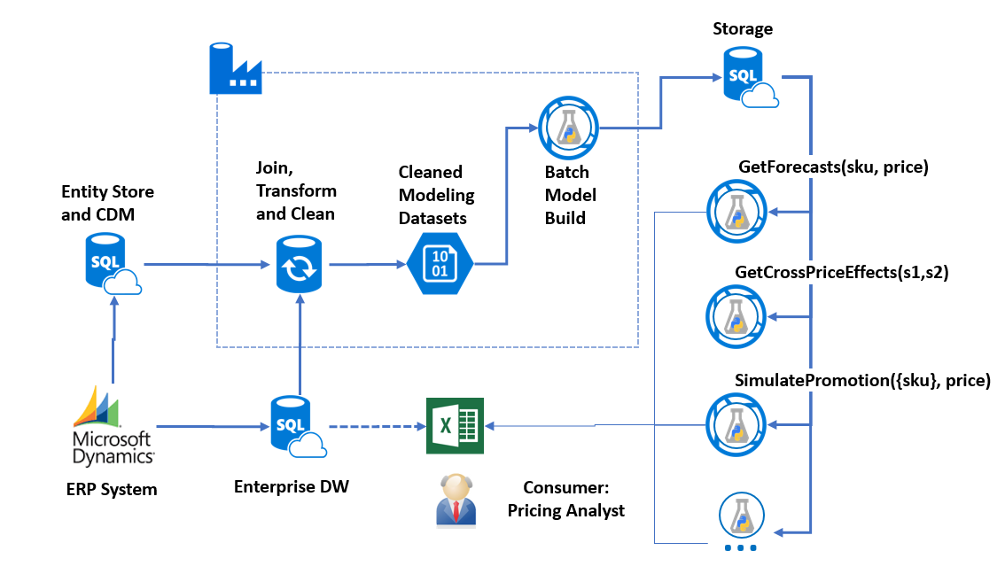
The first (Build) stage of the python code is compute-intensive and takes a few seconds to a few minutes to process, depending on the amount of data. This stage leaves behind .npy (numpy) files in Azure Blob Storage which contain the estimated elasticities, the baseline forecasts, and the intermediate features for each item, site and channel.

The second stage services query the data left in the storage. The files are stored as blobs, and each service first loads the .npy file it needs. Then it answers the question through a lookup in the data structures contained in the file and/or a simple calculation from the elasticity model. This method is currently resulting in RRS latency that is acceptable for interactive use (<2s). As the data grows, we are preparing to output the intermediate data structures into an Azure SQL database, where it will be indexed for constant-time access. Having data in a database will also allow for easier joining and detailed analysis that goes beyond the pre-implemented python services.

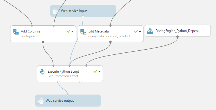
The services themselves are created by deploying a web service from the AzureML Studio. We created wrapper code around the “legacy python” which requires only very short scripts to be deployed into AzureML Execute Python modules in order to create the web services. Most of the code is contained in the PricingEngine python package. The package is included in the script bundle PricingEngine_Python_Dependencies.zip, together with its dependencies (mostly Azure SDK, since sklearn and scipy are already available in the AzureML Python container. The figure below shows the AzureML experiment for GetPromotionEffect - all services are similarly architected.

 

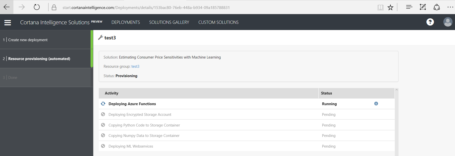
Deployment

The solution is deployed into your Azure subscriptions  through Cortana Intelligence Quick Start (CIQS), currently in private testing. The CIQS is a user friendly wrapper around an Azure Resource Manager template. Please contact us if you would like to try it.

The data science: elasticity model

Core methodology

The core of the engine is an implementation of the idea of “double-residual effect estimation” applied to price elasticity. Price elasticity of an item is simply the derivative of demand wrt price, other things being equal. Other things being never equal, we need counterfactuals for both demand and price. The engine supplied those today as predictions from a carefully elastic-net-regularized linear model, with regularization parameters picked automatically by cross-validation. The elasticity then comes from regressing the demand residual on the price residual.

In addition, various potentially confounding factors are included in the regression:

• Seasonal indicators
• The price itself, in absolute, and relative to other products in the same category
• Lagged changes in price and demand
• The recent trend in the product’s category prices and demands
• Indicator variables for the product category and site, channel
• The recent demand and pricing trends at the site and in the channel
• Indicator variables for the products category
• Various interactions between these variables, especially between price change and site, channel and category

To control the dimensionality of the model when we have large product hierarchies with many categories up to 5 level deep, we use a model stacking approach. We first estimate the model M1 with only the top-level category indicators enabled. We capture the residuals of M1 and for each level-1 category, we fit a model of the residuals, with level-2 category indicators as additional predictors, using only transactions on items from the level-1 category. This process continues recursively, in effect creating a tree of models. Heavy elastic net regularization occurs at each step. Since the hierarchy is up to 5 levels deep, each demand prediction involves running 5 models along the branch of the category tree.

There is a lot more going on. The engine also estimates pull-forward effects (demand shifting to promotion period from subsequent ones). We'll blog more about that in a detailed future post.

Data acquisition and cleaning

A major challenge in development of the model was data cleaning for model fitting purposes – what was the price of oranges on 1/1/2015? Businesses don’t always have the historical offered prices systematically recorded as a dataset and they can be difficult to pull out of the ERP system.

Even when the price history is on hand, it can be surprisingly complicated to answer the question in a B2B context. In B2C context, most customers face one price (but consider coupons and co-branded credit cards!). In B2B, the same item can and does sell at many different prices. The following chart illustrates the sales of one item in one site in time. The x axis is days, the y axis is the volume, and the colors represent different price points.

 

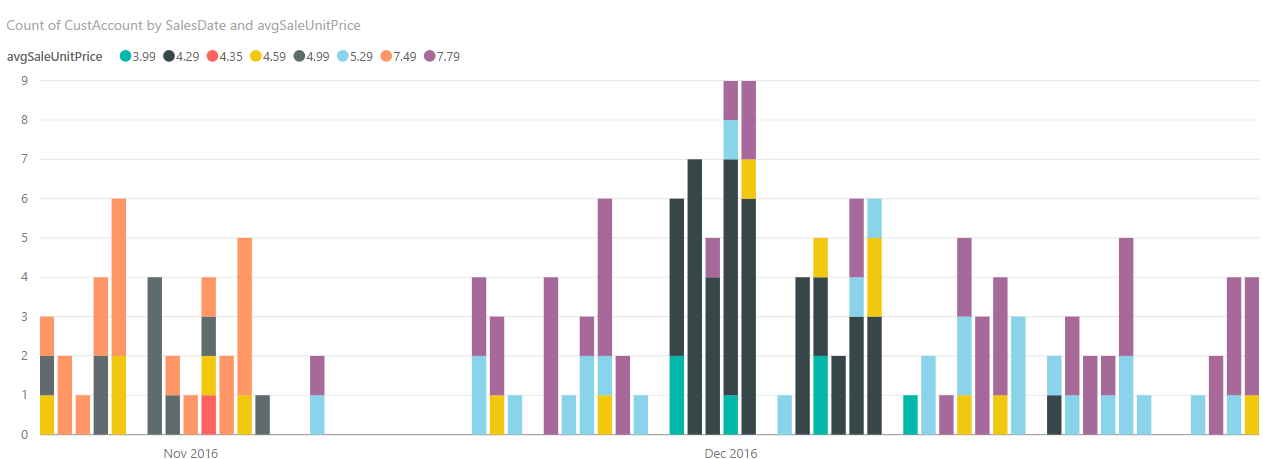
The prices differ because of channels (delivery vs pick-up, internet vs in-person), preexisting pricing agreements, etc. Price variations open us up to the treacherous modeling issue of “composition of demand”. When multiple customer segments pay different prices, the average price is a function of proportion of customers from different segment and can change even if no one is facing a different price. Thus average sales price is a very poor covariate to use for modeling!

With guidance from the customer, we solved both the problem of historical record and the problem of price variation by considering “the price” to be the weekly customer-modal price (the price at which the most customers bought). We exclude items averaging fewer than 3 sales a week from the modeling.

Conclusions

The engine combines strengths of ML, which is good at predicting, with those of econometrics, which is good at preparing training data to mitigate biases and producing causally interpretable models. As a cloud application, it is easy to deploy to your subscription and try out.

Please contact Tomas.Singliar@microsoft.com with questions.