Introducing Microsoft Data Science Virtual Machine

Article
11/21/2016

Microsoft Data Science Virtual Machine (DSVM) is a custom virtual machine on Microsoft's Azure cloud build specifically for doing data science. It's a powerful data science development sandbox equipped with the most popular tools for data exploration and modelling. You can provision a DSVM with a few clicks on Microsoft Azure website, and within 10-20 minutes you will have a running virtual machine to which you can connect via the standard Windows Remote Desktop Connection tool.

DSVM runs on a Windows Server 2012 and contains the following data science and development tools (taken from the product page): "The main tools include Microsoft R Server Developer Edition, Anaconda Python distribution, Jupyter notebooks for Python and R, Visual Studio Community Edition with Python, R and node.js tools, Power BI desktop, SQL Server 2016 Developer edition. It also includes deep learning tools like CNTK (an Open Source Deep Learning toolkit from Microsoft) and mxnet; ML algorithms like xgboost, Vowpal Wabbit. The Azure SDK and libraries on the VM allows you to build your applications using various services in the cloud that are part of the Cortana Analytics Suite which includes Azure Machine Learning, Azure Data Factory, Azure Stream Analytics and SQL Data Warehouse, Hadoop, Azure Data Lake, Spark and more." There is also an equivalent Linux based DSVM.

In this post, we will briefly describe how to provision a data science VM, then go over a simple use case of exploring a large order demand data set using Microsoft R Server. At the end of the post we provide several helpful resources for further reading.

Provisioning a Data Science VM

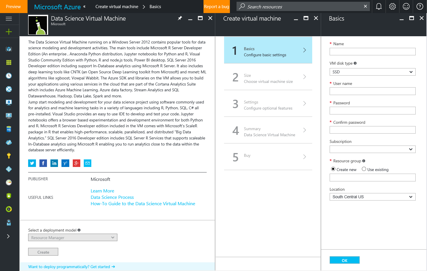
To provision a DSVM, go to Azure portal, and search for New -> Data Science Virtual Machine, and select Create (as shown in the picture below). This will take you through a configuration wizard, asking for inputs, such as Azure subscription and resource group, VM account credentials, VM size, etc. After completing the wizard and selecting the Buy button, it takes 10-20 minutes for the VM to be created and ready for use.

Microsoft R Server

Of particular interest to data scientists who use R for common data science tasks on large data will be Microsoft R Server (MRS) that comes with DSVM. Microsoft R Server is enterprise-class distribution of R that allows for scalable data wrangling and modeling for data that does not fit into available RAM. MRS stores the data in external data frames (xdf) limited only by space on disk in a binary file format that is optimized to work with the MRS libraries. It retrieves data in blocks for efficient reading of arbitrary columns and contiguous rows, and optimizes the block sizes depending on individual computer I/O bandwidth. This results in significant speed-ups with respect to interactive data wrangling and modeling.

To develop R code with Microsoft R Server, we used RStudio, a popular IDE for R, which comes pre-installed on the DSVM.

NOTE: To make sure that RStudio loads MRS (instead of MRO - a more limited distribution of MRS), go to Tools -> Global Options -> General, and change the R Version to point to C:\Program Files\Microsoft SQL Server\130\R_SERVER.

Other popular environments for developing R code available on DSVM are R Tools for Visual Studio and Jupyter Notebooks.

Example use case: exploration of product demand data

In demand forecasting scenarios, the data is commonly very large, with millions or records indicating shipment records, customer orders, or consumption data. If we wanted to explore the data, look at the variable types, distributions, or visualize the demand over time for hints about trends, seasonality, etc., we might run into issues with the base R version, as the data might be larger than the available memory. Let's look at one such example below, where we used Microsoft R Server to explore and visualize such large data.

We downloaded our data set in a .csv format from a sharepoint site onto the VM. One can easily connect to an external data source (sharepoint, Azure blob, Azure SQL database, etc.), and access the data directly from MRS, or download it onto the VM, and access it locally.

Let's import the data into the .xdf format.

 in.file <- file.path('C:/shared/demand_dataset.csv')
xdf.file <- "demand_dataset.xdf"

# Read data from csv 
dataset <- rxImport(inData = in.file,
                    outFile = xdf.file,
                    overwrite = TRUE,
                    type = "text",
                    missingValueString = "N/A",
                    stringsAsFactors = TRUE)

Let's look at the number of rows and columns in our dataset.

 > dim(dataset)
[1] 41034690       20

It's a relatively large data set with 41,034,690 orders and 20 variables describing those orders.

To get information about the variables in the data set, such as variable names, data types, low/high values for numeric variables, unique values and number of unique values for categorical variables, etc., we can run the following command:

 # Get variable info
rxGetVarInfo(dataset)

Due to the privacy of the data, we omit the output here.

Let's look at the summary statistics for the volume variable in our data set.

 > # Get summary stats
> rxSummary(~ volume, data = dataset)

Rows Processed: 41034690 
Call:
rxSummary(formula = ~volume, data = dataset, reportProgress = 1)

Summary Statistics Results for: ~volume
Data: dataset (RxXdfData Data Source)
File name: demand_dataset.xdf
Number of valid observations: 41034690 

Name        Mean     StdDev   Min Max       ValidObs MissingObs
volume      48214.28 219421.2 0   135384480 41034690 0

We can see that the mean order volume was 48,214.28, and the largest order had 135,384,480 volume.

Let's aggregate the volume data and plot it over time. In order to aggregate the data, we will take advantage of R package dplyrXdf, which allows for streamlined and simplified data manipulation.

 # Load dplyrXdf package
library(dplyrXdf)

# Aggregate volume over time (per yyyy-mm-dd)
volume.by.ymd <- dataset %>%
    select(date, volume) %>%
    group_by(date) %>%
    summarise(volume = sum(volume)) %>%
    as.data.frame

# Plot the aggregated data
ggplot(volume.by.ymd, aes(date, volume)) + geom_line() + ggtitle("Daily volume over time")

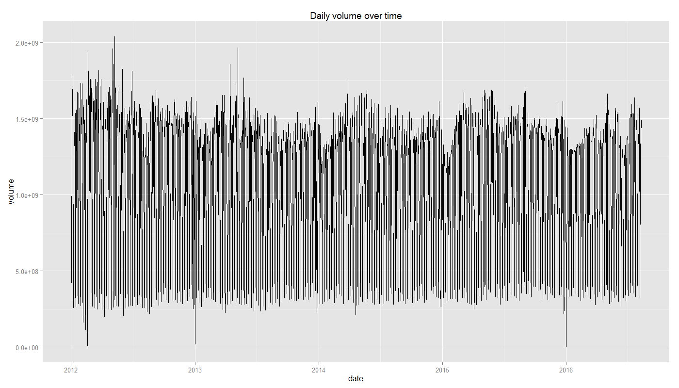
This plot may be too dense to visually inspect and detect any trends in the daily plot, so let's look at the data aggregated at the monthly level.

 # Aggregate volume over time (per yyyy-mm)
volume.by.ym <- volume.by.ymd %>%
    select(date, volume) %>%
    mutate(date = as.Date(as.yearmon(date))) %>%
    group_by(date) %>%
    summarise(volume = sum(volume)) %>%
    as.data.frame

# plot the aggregated data
ggplot(volume.by.ym, aes(date, volume)) + geom_line() + ggtitle("Monthly volume over time")

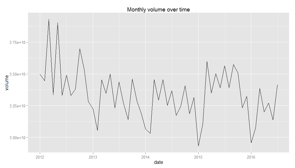
This plot is much clearer and it's easier to see trends and seasonality. There is a decreasing trend in the data in early years, potentially reflecting some changes in data reporting. We can also see a clear seasonal pattern in the data with the major volume dips around the end of each year, reflecting patterns around the winter holidays.

We have shown a simple use case of how to explore a large demand data set using Microsoft R Server on Data Science Virtual Machine. Within less than an hour, we were able to provision a virtual machine with MRS already installed (and other popular data science tools), and gain valuable insights from our data without a need for any deep statistics or machine learning skills.

References

Author: Vanja Paunić, Data Scientist, Microsoft

Introducing Microsoft Data Science Virtual Machine

Provisioning a Data Science VM

Microsoft R Server

Example use case: exploration of product demand data

Further Reading

References

Additional resources