Applying Deep Learning at Cloud Scale, with Microsoft R Server & Azure Data Lake
This post is by Max Kaznady, Data Scientist, Miguel Fierro, Data Scientist, Richin Jain, Solution Architect, T. J. Hazen, Principal Data Scientist Manager, and Tao Wu, Principal Data Scientist Manager, all at Microsoft.
Today's businesses collect vast volumes of images, video, text and other types of data – data which can provide tremendous business value if efficiently processed at scale and using sophisticated machine learning algorithms. There's a growing demand for massively parallel scoring of large production workloads using sophisticated pre-trained models such as Deep Neural Networks (DNNs). Example applications include real-time labeling and monitoring of sentiment in tweets, itemization of equipment and materials at construction sites through video surveillance, and real-time fraud detection in the financial domain, to name a few.
In a previous blog post, we described how to set up DNNs in the cloud using a high performance GPU VM and MXNet. In this sequel, we outline a pipeline process for training and scoring with DNNs in a large-scale production environment. We describe how to pre-process the training set using Microsoft R Server, re-train the MXNet model in the cloud with NVIDIA Tesla K80 GPUs, and finally how to score large datasets stored in Azure Data Lake Store using HDInsight Apache Spark clusters. This approach can be quickly re-iterated with Active Learning to yield successively better results.
We demonstrated this capability recently at the Microsoft Machine Learning & Data Science Summit at Ignite – a video recording of our presentation, "Deep Learning in Microsoft R Server Using MXNet on High-Performance GPUs in the Public Cloud", is available here.
Architecture
In this post, we illustrate how to massively parallelize scoring using a pre-trained DNN machine learning model on an HDInsight Apache Spark cluster. We are seeing a growing number of scenarios that involve the scoring of pre-trained DNNs on a large number of images, such as in Microsoft's partnership with Liebherr to visually recognize objects inside a refrigerator. In this post, we illustrate such scoring on a large-scale synthetic image set created for demonstration purposes.
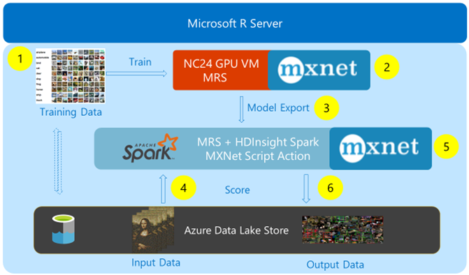
Figure 1: Overview of DNN training and scoring architecture.
The high-level process architecture of our system, as shown in Figure 1, is broken down into the following sequence of steps, shown by the yellow circles:
- Export and preprocessing of training data from Azure Data Lake Store (ADLS) onto Azure N-series NC24 Virtual Machine.
- MXNet DNN model training using NVIDIA Tesla K80 GPU using Microsoft R Server (MRS).
- Export of trained model into the HDInsight Spark edge node filesystem.
- Ingress of test data from ADLS into the HDInsight Spark edge node filesystem.
- Massively parallel scoring through the distribution of the exported model and test data onto the local filesystem of each individual Spark worker node.
- Egress of scored data back to ADLS.
A typical large-scale image scoring scenario may require very high I/O throughput and/or large storage capacity, to which ADLS provides a high performance and scalable solution. Furthermore, ADLS imposes data schema on read, which allows the user to not worry about the schema until the data is needed. From the user's perspective, ADLS functions like any other HDFS storage account through the supplied HDFS connector.
Training occurs on an Azure N-series NC24 GPU-enabled Virtual Machine, which allows training of our DNNs with bare-metal GPU hardware acceleration in the public cloud using as many as four NVIDIA Tesla K80 GPUs.
We use the HDInsight Spark Cluster to massively parallelize the scoring of a large collection of images with the rxExec function in MRS by distributing the workload across the HDInsight Spark worker nodes. The scoring workload is orchestrated from a single instance of MRS and each worker node can read and write data to ADLS independently, in parallel.
To execute MXNet's DNN prediction capabilities on each worker node of the HDInsight Spark cluster in parallel, we launch MXNet out-of-process on each worker node. This requires MXNet to be installed on each worker node of the Spark cluster. HDInsight Spark cluster conveniently comes with the Script Action mechanism, which automates such cluster-wide installations. We have automated the content of our previous blog into a simple BASH script, linked as a Script Action in the HDInsight Spark cluster.
Training and Scoring DNNs
Problem Formulation
We use the 10,000 images in the test set of the CIFAR-10 data set (see Figure 2) and the "metapixel" program to generate a collage of the original high-resolution Mona Lisa painting but using only the images from CIFAR (low-res pictures of both are shown in Figure 3). The resulting collage thus contains thousands of individual images of each of the 10 different object types shown in Figure 3. The goal of our example system is to discover all the tiles of boats and cars among the overlapping tiles which make up the generated collage.
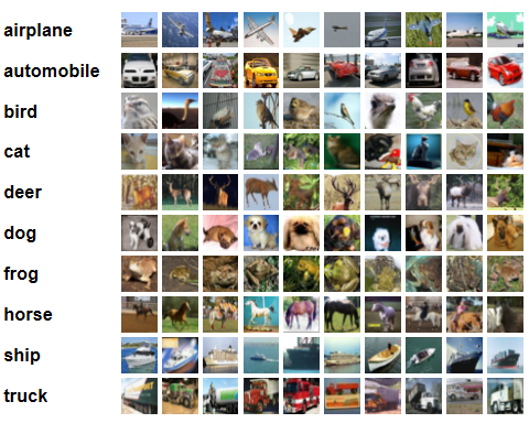
Figure 2: CIFAR-10 dataset, from "Learning Multiple Layers of Features from Tiny Images", by Alex Krizhevsky, 2009.
Such discovery task is hard even for a human; the tiles are small, only 32x32 pixels, so even if they aren't overlapping, it's already difficult to spot all the cars and boats. The task is made even more difficult since overlapping tiles in the collage cover certain regions of the car and boat tiles.


Figure 3: Original high-resolution image of Mona Lisa at the top, and
Mona Lisa collage generated from the CIFAR-10 test dataset using metapixel below.
Machine Learning Model
For the Convolutional Deep Neural Network, we use the Residual Network (ResNet) DNN with 21 convolutional blocks, developed by Microsoft Research (MSR). Note that we cannot directly use the 50,000 basic CIFAR-10 training set tiles to train the ResNet for the following reasons:
- The CIFAR-10 dataset is typically used for image classification, and this is an object detection task (i.e. tagging individual objects present in sub-regions of an image).
- Only partial images of cars and boats are visible in the collage, because the collage creation process causes some images to overlap others.
- Negative examples are very important to obtain an accurate model. In our case the negative examples are the remaining 8 classes which are treated as one giant class.
Data Pre-Processing
We generate three different canvases of training images, where, for each respective training canvas, we randomly scatter:
- Training set images of only cars,
- Training set images of only boats, and
- Negative training set images from the other 8 object categories.
We slice up each training set image canvas in parallel into 32x32 tiles with a step size of 8 pixels in both vertical and horizontal directions from within Microsoft R Server, taking advantage of 24 CPU cores on Azure N-series NC24 VMs as observed in the htop program in Figure 4.
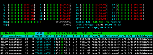
Figure 4: Generating training data in parallel using Microsoft R Server.
As a result of data preprocessing, the training set is inflated from roughly 200MB to 8.9GB of raw 32x32 PNG images from the three training canvases:
- Car class: Original CIFAR-10 training set car images and all generated images of cars overlapping cars.
- Boat class: Original CIFAR-10 training set boat images and all generated images of boats overlapping boats.
- Negatives class: Original CIFAR-10 training set images of negatives and all generated images of negatives overlapping negatives.
Model Training
There are four NVIDIA K80 GPUs available on Azure N-series NC24 VM, so one can easily train multiple models in parallel and also parallelize training across different GPUs as well. In Figure 5 we show the output of the nvidia-smi command for the three MXNet models trained in parallel.
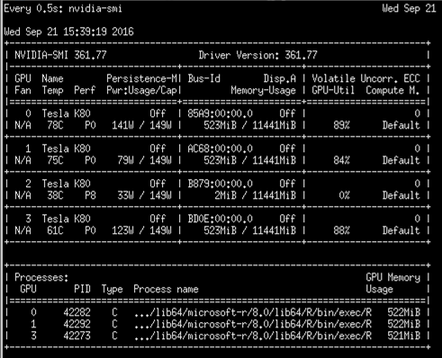
Figure 5: Parallel GPU model training with Microsoft R Server on Azure N-series NC24 VM.
We compress 2.3 million training images from 8.9GB of raw PNG images to 5.1GB with im2rec binary in 10 minutes for optimal training performance. Training takes around 27 minutes for a single epoch with default batch size of 128 images, and just under 20 epochs are needed to obtain over 99.7% accuracy on the training set (we ran for 40 epochs with varying learning rates for 99.99% training set accuracy).
Model Scoring
Scoring performance can be significantly improved by simply increasing the number of HDInsight Spark worker nodes in the Azure Portal. Note that since the Script Action is persisted, MXNet will automatically be installed on any new worker nodes which have been added to the Spark cluster. We illustrate the partitioning used with 12 HDInsight Spark D4 worker nodes in Figure 6 – the test image is sliced into 12 horizontal strips which are processed on each Spark worker node in parallel with a 32x32 sliding window and a step size of 16 pixels. Figure 7 illustrates how easy it is to scale the cluster from the Azure Portal.
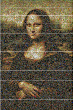
Figure 6: Partitioned test image for parallel scoring on HDInsight Spark cluster.
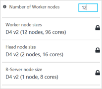
Figure 7: HDInsight Spark with Microsoft R Server cluster scaling options.
Notice that one can process large high-resolution images of arbitrary size in a very short timeframe by simply increasing the number of HDInsight Spark worker nodes, so our scoring performance is truly scalable for very large datasets. For instance, on a single HDInsight Spark worker node, it takes 69.1 minutes to process the test image, but with 12 HDInsight Spark worker nodes it only takes 6.9 minutes to perform the same task. We fall short of the expected 12x speed-up because the image is not divided equally into 12 horizontal strips, so one Spark executor will always take slightly longer to process the remainder.
Results
Each worker node returns a labelled list of moving window tile coordinates, which is then used to label the final test image in MRS running on HDInsight Spark edge node. We present the final tagged test image in Figure 8 where cars and boats are labeled with red and green bounding boxes respectively; you can also download the image here. Notice that there are areas which have multiple bounding boxes – this is because each part of the moving window overlapped a part of the car or a boat, and so multiple search windows fired with high confidence on the same object – in this case we used a default classification threshold of 90%. In a production environment problem, post-processing is usually required to select the best region for each object.

Figure 8: Zoomed-out view of the tagged test image.
With enough effort, one can probably find plenty of false positive and false negative areas in Figure 8, as well as misclassifications, i.e. cars being classified as boats and vice versa. In a production environment, one can use Active Learning techniques to refine the training set further by learning from test set errors, retraining the model with the enhanced training set to achieve optimal performance on the test set.
Conclusion
This post demonstrated how to tackle a production-scale workload on the public cloud using Azure N-series GPU Virtual Machines to train a deep residual neural network model for parallel image tagging on HDInsight Spark clusters with Microsoft R Server and MXNet, with Azure Data Lake Store being used for data storage and access.
In our next post in this series, we will show how to use multiple GPUs in the public cloud to massively parallelize training on the ImageNet competition dataset by using a multi-layer residual neural network implementation in MXNet.
Max, Miguel, Richin, TJ and Tao.
Acknowledgements
We wish to thank the following team members who contributed to this work:
- Azure ML: Patrick Buehler and Vivek Gupta.
- Azure GPU VM: Huseyin Yildiz and Karan Batta.
- Azure Data Science Virtual Machine: Paul Shealy and Gopi Kumar.
- Microsoft R Server: Mario Inchiosa, Yunshan Zhu and Jianhui Wu.
- MXNet core development team: Qiang Kou (Indiana University) and Tianqi Chen (University of Washington).