Hearing AI: Getting Started with Deep Learning for Audio on Azure
This post is authored by Xiaoyong Zhu, Program Manager, Max Kaznady, Senior Data Scientist, and Gilbert Hendry, Senior Data Scientist, at Microsoft.
There are an increasing number of useful applications of machine learning and Artificial Intelligence in the domain of audio, such as in home surveillance (e.g. detecting glass breaking and alarm events); security (e.g. detecting sounds of explosions and gun shots); driverless cars (sound event detection for increased safety); predictive maintenance (forecast machine failures in a manufacturing process based on vibrations); for real-time translation in Skype and even for music synthesis.
The human brain processes such a wide variety of sounds so effortlessly – be it the bark of puppies, audible alarms from smoke or carbon monoxide detectors, or people talking loudly in a coffee shop – that most of us tend to take this faculty for granted. But what if we could apply AI to help people who are deaf or experience hearing loss achieve something similar? That would be something special.
So, is AI ready to help people who are deaf or experience hearing loss understand and react to the world around them?
In this post, we describe how to train a Deep Learning model on Microsoft Azure for sound event detection on the Urban Sounds dataset, and provide an overview of how to work with audio data, along with links to Data Science Virtual Machine (DSVM) notebooks. All code associated with this post is available on GitHub in Notebook format.
Audio and Speech Processing Basics
It is important to first understand the theory behind audio processing, so we've provided a notebook pre-loaded on DSVM for this purpose, available here, and we explain more advanced concepts here.
Featurization
Before we can perform data science on audio signals, we first need to convert them into a format that is useful for ML algorithms – this process is called featurization.
Audio by itself usually comes in amplitude representation, where the amplitude of the sound changes at a certain frequency over time. This is most convenient for playback. What we need to do is extract the frequencies that are present in each unit of time – the spectrum of frequencies that, when combined, create sounds. Think of playing piano notes – each note resonates at a particular frequency and those frequencies combine to create a particular tune. If we know what notes are being played, we can attempt to classify a piano piece. We therefore need a mechanism of breaking down amplitude over time over frequencies over time: such representation is also commonly called a spectrogram.
A method called the Fast Fourier Transform algorithm (FFT) does just that: it converts amplitude over each time segment into corresponding frequencies. The Nyquist-Shannon sampling theorem states that if we sample the incoming sound signal at a certain rate, we can achieve what's commonly called lossless audio, i.e. we can convert amplitude into frequencies over time and then recover the original amplitude with no error at any point of time from the broken down frequencies. Based on the theorem, if the highest frequency component in a signal is fmax, the sampling rate must be at least 2fmax. The higher fmax is, the higher the bandwidth of the signal. Examples of reasonable sampling rates are 16k for speech and 40k for general audio detection.
Putting Things Together
For dynamic sounds like speech or environment sounds, the frequency spectrum of the audio signal changes over time. We are interested in capturing how these frequencies change, so we apply a method called windowing, where we calculate the FFT over a fixed-length audio sample that shifts in time. The frequency profiles for these samples are then strung together to form a time-series.
To see an example of audio featurization, we can follow this process:
- Wave plot: We generate a sample mono audio clip with only two frequencies present (Figure 1) – this is equivalent to playing two pitch forks for 1 second. We want to show how to recover the two frequencies which we generated and how to featurize them for Deep Learning. This forms a simple base case to check that our featurizer works as expected.
- We then use the FFT to recover the frequencies present in each window:
- The Hamming window function is used during FFT computation (middle plot in Figure 1). The assumption is that the time domain signal is periodic which results in discontinuity at the edges of the FFT window (chunk). Window functions are designed to avoid this, by making sure that the data at the edges is zero (no discontinuity). This is achieved by multiplying the signal by the window function (Hamming in this case) which gradually decays the signal towards zero at the edges.
- Next, we compute the Mel Spectrogram, which is simply the FFT of each audio chunk (defined by sliding window) mapped to mel scale, which perceptually makes pitches to be of equal distance from one another (the human ear focuses on certain frequencies, so our perception is that the mel frequencies are of equal distance from each other). In Figure 1 you can clearly see that we recovered the original frequencies which we entered at the beginning of this notebook with no loss – two frequencies are present for the entire duration of the audio clip – they show up as bands in the middle and rightmost subplots.
- This is the raw featurization which is needed to detect acoustic events in audio (e.g. dog barking, water boiling, tires screeching), which is our ultimate goal. For human speech recognition systems, this featurization is not usually used directly, as human brains tend to focus on lower-frequency patterns in audio, so the featurization approach needs to go a step further and compute Mel Frequency Cepstral Coefficients (MFCC). If you're curious, the details of this computation can be found in this sample notebook.
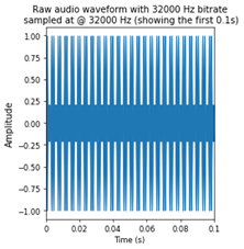
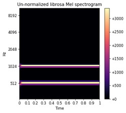
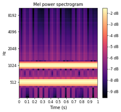
Figure 1: Sound wave, frequency domain and log mel scaled frequency domains of generated audio waves.
Dataset
In this post, we will use the publicly available UrbanSound8K dataset. This dataset contains 8,732 labeled 4-second sound excerpts of urban sounds from 10 classes: air conditioner, car horn, children playing, dog barking, drilling, engine idling, gunshot, jackhammer, siren, and street music. The classes are drawn from the urban sound taxonomy. You can directly download the data from the website: https://serv.cusp.nyu.edu/projects/urbansounddataset/urbansound8k.html.
Setting up a Deep Learning Virtual Machine in Azure
Data Science VM on Azure helps jumpstart your deep learning projects. It already handles tasks such as GPU driver installation, deep learning framework setup, and environment configuration. Users can just provision a new DSVM and get productive from the get go (exact steps are described here).
Preprocessing the Data and Generating Spectrograms
Below is an illustration of a certain dog barking. The picture on the left is the audio file in the temporal domain, where the horizontal axis stands for the time, and the vertical axis stands for the amplitude for the audio file in a timestamp, with each peak featurizing each distinct bark.
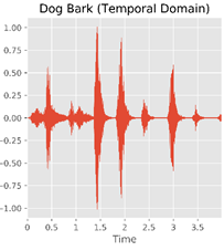
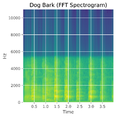
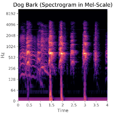
Figure 2: Dog barking in different domains. Left: Normalized amplitude in time domain; Middle: FFT spectrogram; Right: Log of FFT spectrogram in Mel-scale.
We use the same process as described above to test our base case example of two frequencies to featurize the UrbanSounds8K dataset – the final featurization is shown in the plot on the right of Figure 2.
The choice of the length of the sliding window used to featurize the data into a mel-spectrogram is empirical – based on Environmental sound classification with convolutional neural networks paper by Piczak, longer windows seem to perform better than shorter windows. In this post, we will use a sliding window with a length of 2 seconds with a 1 second overlap; this will also determine the length of each audio sample's time series.
We also need to choose the number of frequency bands, i.e. the resolution of the frequency axis. The number of frequency bands has a physical meaning – we cannot increase the number of frequency bands arbitrarily. For example, if we choose a small number of bands, say 10, when calculating the spectrogram, the spectral resolution will only be 10 units and the spectrogram will lose a lot of information (see the image at the left in Figure 3 – it has a very coarse representation of the original audio signal). On the other hand, if we choose too many bands, such as 1000 (the figure on the right), we will have a high-resolution image, but there will be many empty bands since we under-sample the signal within each band (not enough data samples per frequency band given the fixed bitrate of our audio) – this is shown by the empty black regions in the spectrogram. Choosing the number of bands is somewhat empirical too, and in this case, we choose 150 bands – a widely used number in many papers.
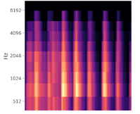
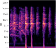
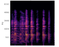
Figure 3: Choosing appropriate bands for mel-spectrogram calculation. Left: Process with 10 bands; Middle: Process with 150 bands; Right: Process with 1000 bands.
Building the Convolutional Neural Network (CNN) for Audio
We use the same DNN architecture on featurized data as the winning solution to DCASE 2016 Track 4. DCASE is the audio challenge for sound domain and is held every year. The technical report which details the winning solution can be found here. The DNN architecture is similar to the popular VGG network in terms of having many convolutional layers but less parameters in each layer, which makes the model "deep and narrow" (there are also wide and shallow approaches which can be used). Compared to the original VGG network, this DCASE winner network shrinks to 11 Convolutional layers and adds a few Batch Normalization layers for faster convergence and to make sure the gradients are passed efficiently during back-propagation.

Figure 4: Model architecture.
We use Keras to build up the model. Keras is famous for its simple yet powerful APIs, and it acts as a higher-level API on top of TensorFlow, Cognitive Toolkit (CNTK), or Theano.
A Note on Loading Data
Although we load all the data at once in the GitHub repo, and feed a big array to the classifier, one thing that is commonly done is to load data iteratively in chunks and to perform any data augmentation as needed on each chunk, especially for large datasets such as ImageNet. As you can imagine, since we are mainly using GPUs for neural network training, the CPU resources are used to load and transform data.
For image data you can perform real-time data augmentation using CPUs, for example shearing, cropping, flipping, etc. However, for our spectrogram this doesn't make much sense, as each pixel in our spectrogram has some physical meaning. Flipping a cat picture will still make it a cat, while flipping spectrograms will likely change its underlying physical meaning. People also attempted other data augmentation techniques such as changing pitches of the sound file, but for simplicity we just use the raw mel-spectrograms here without augmenting the data. You can learn more details on audio data augmentation in the "Improving Model Performance" section below.
Training the Model
After we have defined the model, we will need to compile and fit it on the training dataset. Compilation requires us to specify a few parameters: the optimizer that we want to use, the loss function, and the metrics. In this case, we will use the popular "Adam" optimizer, which is short for "adaptive moment estimation". This blog post on gradient descent optimization algorithms provides a nice overview and visualization for popular optimization algorithms including Adam.
We use categorical cross entropy as the loss function, which is widely used in classification problems. We also use the accuracy of the model as the metrics. Figure 5 shows the accuracy of the model as the number of times the dataset is completely processed (epochs), where you can see that the validation accuracy converges around 78%. On the test set, we were able to obtain average accuracy of over 78% with the standard deviation of 4.6% - this result is quite good, comparable to the state-of-art result from the Learning from Between-class Examples for Deep Sound Recognition paper. Your results should be close to our results when you re-run the notebook on DS VM; even though we fixed the random seed, due to multi-threading and cuDNN implementation, Keras is not guaranteed to produce identical results each time. Notebooks should work with both TensorFlow and CNTK back ends.
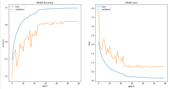
Figure 5: Accuracy (left) and loss (right) changes across different epochs.
Test Set Performance Metrics
Since this is a typical classification problem, we also want to visualize the confusion matrix to visualize the classification performance for each class. For example, the model might be good at detecting dog barking sounds but might be poor at detecting gun shots. We want to look at the model performance across each class and at the overall accuracy across all classes. Figure 6 shows the confusion matrix for the model we have trained:
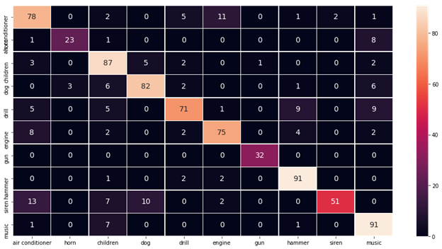
Figure 6: Test set confusion matrix with over 78% accuracy.
The horizontal axis represents the actual true class, and the vertical axis represents the ones predicted by our model. From the matrix, looks like our model is good at most of the classes, but for "children playing" and "hammer" classes, there are many misclassifications. As a next step, we need to improve the performance of the model.
Improving Model Performance
There are certainly many additional techniques that we can apply to get better performance. In a recent paper called Learning from Between-class Examples for Deep Sound Recognition (under review for ICLR 2018), the author shows how between-class learning can significantly improve the performance.
Data augmentation is known to work well in image data set, however Piczak's paper suggests that simple data augmentation for audio (such as changing the pitch) does not improve the result much. In the GitHub repository we use a scaler for the spectrograms and it increases the accuracy of the model.
Conclusion
In this blog post, we introduced the audio domain and showed how to utilize audio data in machine learning. We demonstrated how to build a sound classification Deep Learning model and how to improve its performance. All the code is available on GitHub, and you can provision a Data Science Virtual Machine to try it out.
Xiaoyong, Max & Gilbert