Tutorial: Forecast demand with no-code automated machine learning in the Azure Machine Learning studio

Learn how to create a time-series forecasting model without writing a single line of code using automated machine learning in the Azure Machine Learning studio. This model predicts rental demand for a bike sharing service.

You don't write any code in this tutorial, you use the studio interface to perform training. You learn how to do the following tasks:

• Create and load a dataset.
• Configure and run an automated ML experiment.
• Specify forecasting settings.
• Explore the experiment results.
• Deploy the best model.

Also try automated machine learning for these other model types:

• For a no-code example of a classification model, see Tutorial: Create a classification model with automated ML in Azure Machine Learning.
• For a code first example of an object detection model, see the Tutorial: Train an object detection model with AutoML and Python.

Prerequisites

• An Azure Machine Learning workspace. See Create workspace resources.

• Download the bike-no.csv data file

Sign in to the studio

For this tutorial, you create your automated ML experiment run in Azure Machine Learning studio, a consolidated web interface that includes machine learning tools to perform data science scenarios for data science practitioners of all skill levels. The studio isn't supported on Internet Explorer browsers.

1. Sign in to Azure Machine Learning studio.

2. Select your subscription and the workspace you created.

3. Select Get started.

4. In the left pane, select Automated ML under the Author section.

5. Select +New automated ML job.

Create and load dataset

Before you configure your experiment, upload your data file to your workspace in the form of an Azure Machine Learning dataset. Doing so, allows you to ensure that your data is formatted appropriately for your experiment.

1. On the Select dataset form, select From local files from the +Create dataset drop-down.

   1. On the Basic info form, give your dataset a name and provide an optional description. The dataset type should default to Tabular, since automated ML in Azure Machine Learning studio currently only supports tabular datasets.

   2. Select Next on the bottom left

   3. On the Datastore and file selection form, select the default datastore that was automatically set up during your workspace creation, workspaceblobstore (Azure Blob Storage). This is the storage location where you upload your data file.

   4. Select Upload files from the Upload drop-down.

   5. Choose the bike-no.csv file on your local computer. This is the file you downloaded as a prerequisite.

   6. Select Next

      When the upload is complete, the Settings and preview form is pre-populated based on the file type.

   7. Verify that the Settings and preview form is populated as follows and select Next.

      Field	Description	Value for tutorial
      File format	Defines the layout and type of data stored in a file.	Delimited
      Delimiter	One or more characters for specifying the boundary between  separate, independent regions in plain text or other data streams.	Comma
      Encoding	Identifies what bit to character schema table to use to read your dataset.	UTF-8
      Column headers	Indicates how the headers of the dataset, if any, will be treated.	Only first file has headers
      Skip rows	Indicates how many, if any, rows are skipped in the dataset.	None

   8. The Schema form allows for further configuration of your data for this experiment.

      1. For this example, choose to ignore the casual and registered columns. These columns are a breakdown of the cnt column so, therefore we don't include them.

      2. Also for this example, leave the defaults for the Properties and Type.

      3. Select Next.

   9. On the Confirm details form, verify the information matches what was previously populated on the Basic info and Settings and preview forms.

   10. Select Create to complete the creation of your dataset.

   11. Select your dataset once it appears in the list.

   12. Select Next.

Configure job

After you load and configure your data, set up your remote compute target and select which column in your data you want to predict.

1. Populate the Configure job form as follows:

   1. Enter an experiment name: automl-bikeshare

   2. Select cnt as the target column, what you want to predict. This column indicates the number of total bike share rentals.

   3. Select compute cluster as your compute type.

   4. Select +New to configure your compute target. Automated ML only supports Azure Machine Learning compute.

      1. Populate the Select virtual machine form to set up your compute.

         Field	Description	Value for tutorial
         Virtual machine tier	Select what priority your experiment should have	Dedicated
         Virtual machine type	Select the virtual machine type for your compute.	CPU (Central Processing Unit)
         Virtual machine size	Select the virtual machine size for your compute. A list of recommended sizes is provided based on your data and experiment type.	Standard_DS12_V2

      2. Select Next to populate the Configure settings form.

         Field	Description	Value for tutorial
         Compute name	A unique name that identifies your compute context.	bike-compute
         Min / Max nodes	To profile data, you must specify one or more nodes.	Min nodes: 1 Max nodes: 6
         Idle seconds before scale down	Idle time before the cluster is automatically scaled down to the minimum node count.	120 (default)
         Advanced settings	Settings to configure and authorize a virtual network for your experiment.	None

      3. Select Create to get the compute target.

         This takes a couple minutes to complete.

      4. After creation, select your new compute target from the drop-down list.

   5. Select Next.

Select forecast settings

Complete the setup for your automated ML experiment by specifying the machine learning task type and configuration settings.

1. On the Task type and settings form, select Time series forecasting as the machine learning task type.

2. Select date as your Time column and leave Time series identifiers blank.

3. The Frequency is how often your historic data is collected. Keep Autodetect selected.

5. The forecast horizon is the length of time into the future you want to predict. Deselect Autodetect and type 14 in the field.

6. Select View additional configuration settings and populate the fields as follows. These settings are to better control the training job and specify settings for your forecast. Otherwise, defaults are applied based on experiment selection and data.

   Additional configurations	Description	Value for tutorial
   Primary metric	Evaluation metric that the machine learning algorithm will be measured by.	Normalized root mean squared error
   Explain best model	Automatically shows explainability on the best model created by automated ML.	Enable
   Blocked algorithms	Algorithms you want to exclude from the training job	Extreme Random Trees
   Additional forecasting settings	These settings help improve the accuracy of your model. Forecast target lags: how far back you want to construct the lags of the target variable Target rolling window: specifies the size of the rolling window over which features, such as the max, min and sum, is generated.	Forecast target lags: None Target rolling window size: None
   Exit criterion	If a criteria is met, the training job is stopped.	Training job time (hours): 3 Metric score threshold: None
   Concurrency	The maximum number of parallel iterations executed per iteration	Max concurrent iterations: 6

   Select Save.

7. Select Next.

8. On the [Optional] Validate and test form,

   1. Select k-fold cross-validation as your Validation type.
   2. Select 5 as your Number of cross validations.

Run experiment

To run your experiment, select Finish. The Job details screen opens with the Job status at the top next to the job number. This status updates as the experiment progresses. Notifications also appear in the top right corner of the studio, to inform you of the status of your experiment.

Important

Preparation takes 10-15 minutes to prepare the experiment job. Once running, it takes 2-3 minutes more for each iteration.

In production, you'd likely walk away for a bit as this process takes time. While you wait, we suggest you start exploring the tested algorithms on the Models tab as they complete.

Explore models

Navigate to the Models tab to see the algorithms (models) tested. By default, the models are ordered by metric score as they complete. For this tutorial, the model that scores the highest based on the chosen Normalized root mean squared error metric is at the top of the list.

While you wait for all of the experiment models to finish, select the Algorithm name of a completed model to explore its performance details.

The following example navigates to select a model from the list of models that the job created. Then, you select the Overview and the Metrics tabs to view the selected model's properties, metrics and performance charts.

Deploy the model

Automated machine learning in Azure Machine Learning studio allows you to deploy the best model as a web service in a few steps. Deployment is the integration of the model so it can predict on new data and identify potential areas of opportunity.

For this experiment, deployment to a web service means that the bike share company now has an iterative and scalable web solution for forecasting bike share rental demand.

Once the job is complete, navigate back to parent job page by selecting Job 1 at the top of your screen.

In the Best model summary section, the best model in the context of this experiment, is selected based on the Normalized root mean squared error metric.

We deploy this model, but be advised, deployment takes about 20 minutes to complete. The deployment process entails several steps including registering the model, generating resources, and configuring them for the web service.

1. Select the best model to open the model-specific page.

2. Select the Deploy button located in the top-left area of the screen.

3. Populate the Deploy a model pane as follows:

   Field	Value
   Deployment name	bikeshare-deploy
   Deployment description	bike share demand deployment
   Compute type	Select Azure Compute Instance (ACI)
   Enable authentication	Disable.
   Use custom deployment assets	Disable. Disabling allows for the default driver file (scoring script) and environment file to be autogenerated.

   For this example, we use the defaults provided in the Advanced menu.

4. Select Deploy.

   A green success message appears at the top of the Job screen stating that the deployment was started successfully. The progress of the deployment can be found in the Model summary pane under Deploy status.

Once deployment succeeds, you have an operational web service to generate predictions.

Proceed to the Next steps to learn more about how to consume your new web service, and test your predictions using Power BI's built in Azure Machine Learning support.

Clean up resources

Deployment files are larger than data and experiment files, so they cost more to store. Delete only the deployment files to minimize costs to your account, or if you want to keep your workspace and experiment files. Otherwise, delete the entire resource group, if you don't plan to use any of the files.

Delete the deployment instance

Delete just the deployment instance from the Azure Machine Learning studio, if you want to keep the resource group and workspace for other tutorials and exploration.

1. Go to the Azure Machine Learning studio. Navigate to your workspace and on the left under the Assets pane, select Endpoints.

2. Select the deployment you want to delete and select Delete.

3. Select Proceed.

Delete the resource group

Important

The resources that you created can be used as prerequisites to other Azure Machine Learning tutorials and how-to articles.

If you don't plan to use any of the resources that you created, delete them so you don't incur any charges:

1. In the Azure portal, select Resource groups on the far left.

2. From the list, select the resource group that you created.

3. Select Delete resource group.

   

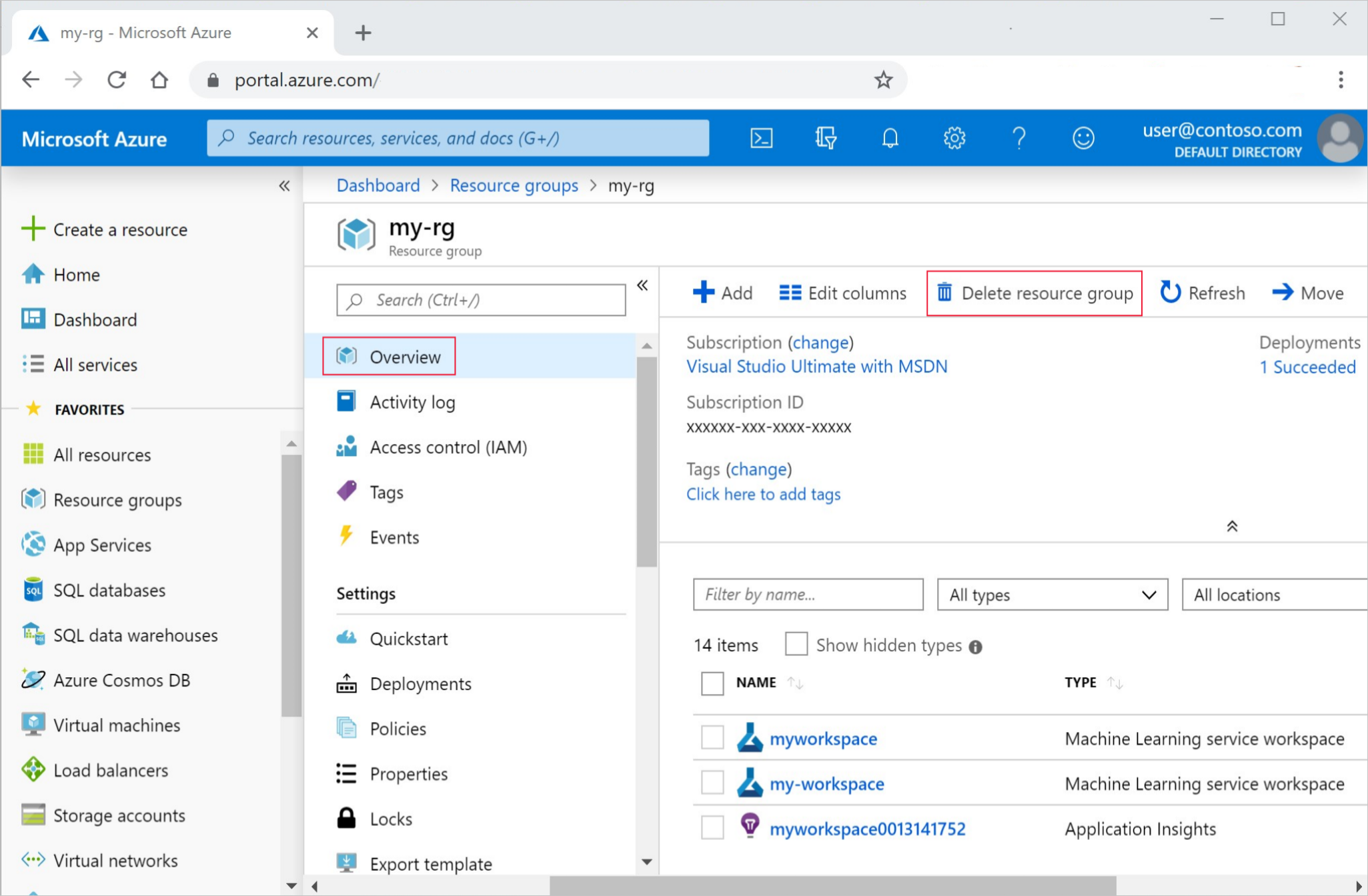
4. Enter the resource group name. Then select Delete.

Next steps

In this tutorial, you used automated ML in the Azure Machine Learning studio to create and deploy a time series forecasting model that predicts bike share rental demand.

See this article for steps on how to create a Power BI supported schema to facilitate consumption of your newly deployed web service:

Consume a web service

• Learn more about automated machine learning.
• For more information on classification metrics and charts, see the Understand automated machine learning results article.

Note

This bike share dataset has been modified for this tutorial. This dataset was made available as part of a Kaggle competition and was originally available via Capital Bikeshare. It can also be found within the UCI Machine Learning Database.

Source: Fanaee-T, Hadi, and Gama, Joao, Event labeling combining ensemble detectors and background knowledge, Progress in Artificial Intelligence (2013): pp. 1-15, Springer Berlin Heidelberg.