Running distributed analyses using RevoScaleR
Important
This content is being retired and may not be updated in the future. The support for Machine Learning Server will end on July 1, 2022. For more information, see What's happening to Machine Learning Server?
Many RevoScaleR functions support parallelization. On a standalone multi-core server, functions that are multithreaded run on all available cores. In an rxSparkConnect or RxHadoop remote compute context, multithreaded analyses run on all data nodes having the RevoScaleR engine.
RevoScaleR can structure an analysis for parallel execution with no additional configuration on your part, assuming you set the compute context. Setting the compute context to rxSparkConnect or RxHadoopMR tells RevoScaleR to look for data nodes. In contrast, using the default local compute context tells the engine to look for available processors on the local machine.
Note
RevoScaleR also runs on R Client. On R Client, RevoScaleR is limited to two threads for processing and in-memory datasets. To avoid paging data to disk, R Client is engineered to ignore the blocksPerRead argument, which results in all data being read into memory. If your datasets exceed memory, you should push the compute context to a server instance on a supported platform (Hadoop, Linux, Windows, SQL Server).
Given a registered a distributed compute context, the following functions can perform distributed computations:
rxSummaryrxLinModrxLogitrxGlmrxCovCor(and its convenience functions,rxCov,rxCor, andrxSSCP)rxCubeandrxCrossTabsrxKmeansrxDTreerxDForestrxBTreesrxNaiveBayesrxExec
Except for rxExec, we refer to these functions as the RevoScaleR high-performance analytics, or HPA functions.
The exception, rxExec, is used to execute an arbitrary function on specified nodes (or cores) of your compute context. It can be used for traditional high-performance computing functions. The rxExec function offers great flexibility in how arguments are passed, so that you can specify that all nodes receive the same arguments, or provide different arguments to each node.
rxPredict on a cluster is only redistributed if the data file is split.
Obtain node information
You can use informational functions, such as rxGetInfo and rxGetVarInfo, to confirm data availability. Before beginning data analysis, you can use rxGetInfo to confirm the data set is available on the compute resources.
You can request basic information about a data set from each node using the rxGetInfo function. Assuming a data source named "airData", you can call rxGetInfo as follows:
rxGetInfo(data=airData)
Note
To load a dataset, use AirOntime2012.xdf from the data set download site and make sure it is in your dataPath. You can then run airData <- RxXdfData("AirOnTime2012.xdf") to load the data on a cluster.
On a five-node cluster, the call to rxGetInfo returns the following:
$CLUSTER_HEAD2
File name: C:\data-RevoScaleR-AcceptanceTest\AirOnTime2012.xdf
Number of observations: 6096762
Number of variables: 46
Number of blocks: 31
Compression type: zlib

$COMPUTE10
File name: C:\data-RevoScaleR-AcceptanceTest\AirOnTime2012.xdf
Number of observations: 6096762
Number of variables: 46
Number of blocks: 31
Compression type: zlib

$COMPUTE11
File name: C:\data-RevoScaleR-AcceptanceTest\AirOnTime2012.xdf
Number of observations: 6096762
Number of variables: 46
Number of blocks: 31
Compression type: zlib

$COMPUTE12
File name: C:\data-RevoScaleR-AcceptanceTest\AirOnTime2012.xdf
Number of observations: 6096762
Number of variables: 46
Number of blocks: 31
Compression type: zlib

$COMPUTE13
File name: C:\data-RevoScaleR-AcceptanceTest\AirOnTime2012.xdf
Number of observations: 6096762
Number of variables: 46
Number of blocks: 31
Compression type: zlib
This confirms that our data set is in fact available on all nodes of our cluster.
Obtain a Data Summary
The rxSummary function returns summary statistics on a data set, including datasets that run in a distributed context.
When you run one of RevoScaleR’s HPA functions in a distributed compute context, it automatically distributes the computation among the available compute resources and coordinates the returned values to create the final return value.
Assuming a job is waiting (or blocking), control is not returned until a computation is complete. We assume that the airline data has been copied to the appropriate data directory on all the computing resources and its location specified by the airData data source object.
Note
The blocksPerRead argument is ignored if script runs locally using R Client.
For example, we start by taking a summary of three variables from the airline data:
rxSummary(~ ArrDelay + CRSDepTime + DayOfWeek, data=airData,
	blocksPerRead=30)
We get the following results (identical to what we would have gotten from the same command in a local compute context):
Call:
rxSummary(formula = ~ArrDelay + CRSDepTime + DayOfWeek, data = airData,
	blocksPerRead = 30)

Summary Statistics Results for: ~ArrDelay + CRSDepTime + DayOfWeek
Data: airData (RxXdfData Data Source)
File name: /var/RevoShare/v7alpha/aot12
Number of valid observations: 6096762

	Name       Mean      StdDev    Min           Max        ValidObs MissingObs
	ArrDelay    3.155596 35.510870 -411.00000000 1823.00000 6005381  91381
	CRSDepTime 13.457386  4.707193    0.01666667   23.98333 6096761      1

Category Counts for DayOfWeek
Number of categories: 7
Number of valid observations: 6096762
Number of missing observations: 0

	DayOfWeek Counts
	Mon       916747
	Tues      871412
	Wed       883207
	Thur      905827
	Fri       910135
	Sat       740232
	Sun       869202
Perform an rxCube computation
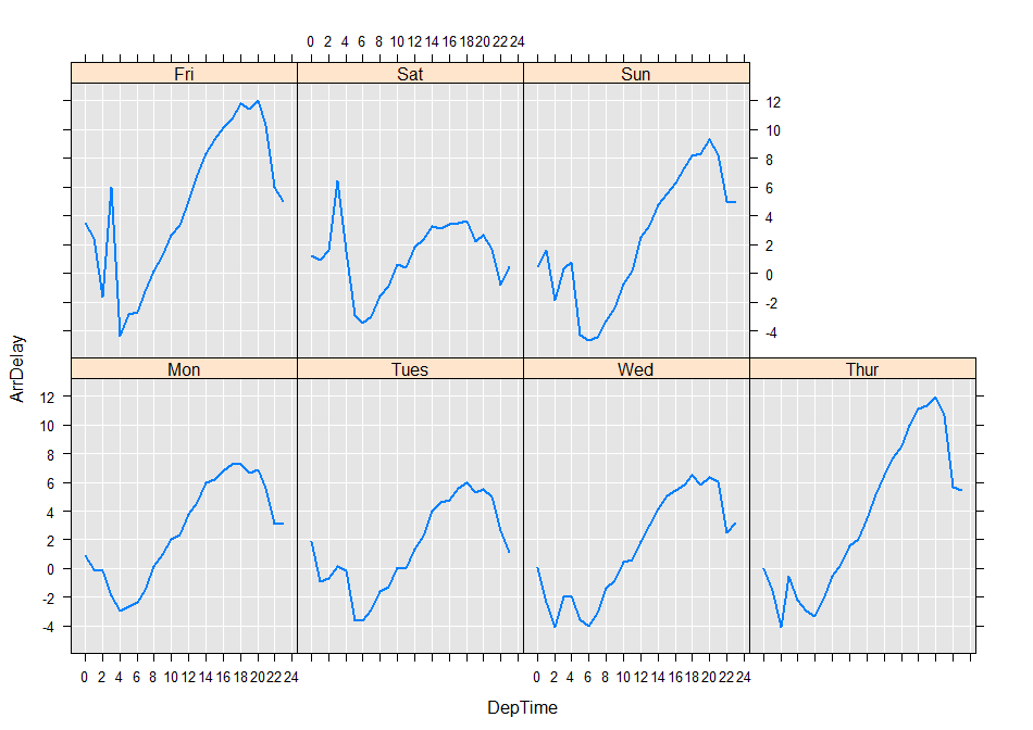
We can perform an rxCube computation using the same data set to compute the average arrival delay for departures for each hour of the day for each day of the week. Again, the code is identical to the code used when performing the computations on a single computer, as are the results.
delayArrCube <- rxCube(ArrDelay ~ F(CRSDepTime):DayOfWeek,
	data=airData, blocksPerRead=30)
Note
The blocksPerRead argument is ignored if script runs locally using R Client.
Notice that in this case we have returned an rxCube object. We can use this object locally to, for example, extract a data frame and plot the results:
plotData <- rxResultsDF( delayArrCube )
names(plotData)[1] <- "DepTime"
rxLinePlot(ArrDelay~DepTime|DayOfWeek, data=plotData)
Perform an rxCrossTabs computation
The rxCrossTabs function provides essentially the same computations as rxCube, but presents the results in a more traditional cross-tabulation. Here we look at late flights (those whose arrival delay is 15 or greater) by late departure and day of week:
crossTabs <- rxCrossTabs(formula = ArrDel15 ~ F(DepDel15):DayOfWeek,
							data = airData, means = TRUE)
crossTabs
which yields:
Call:
rxCrossTabs(formula = ArrDel15 ~ F(DepDel15):DayOfWeek, data = airData,
	means = TRUE)

Cross Tabulation Results for: ArrDel15 ~ F(DepDel15):DayOfWeek
Data: airData (RxXdfData Data Source)
File name: /var/RevoShare/v7alpha/AirlineOnTime2012
Dependent variable(s): ArrDel15
Number of valid observations: 6005381
Number of missing observations: 91381
Statistic: means

ArrDel15 (means):
			DayOfWeek
F_DepDel15        Mon       Tues        Wed       Thur        Fri        Sat
			0 0.04722548 0.04376271 0.04291565 0.05006577 0.05152312 0.04057934
			1 0.79423651 0.78904905 0.79409615 0.80540551 0.81086142 0.76329539
			DayOfWeek
F_DepDel15        Sun
			0 0.04435956
			1 0.79111488
Compute a Covariance or Correlation Matrix
The rxCovCor function is used to compute covariance and correlation matrices; the convenience functions rxCov, rxCor, and rxSSCP all depend upon it and are usually used in practical situations. For examples, see Correlation and variance/covariance matrices.
The following example shows how the main function can be used directly:
covForm <- ~ DepDelayMinutes + ArrDelayMinutes + AirTime
cov <- rxCovCor(formula = covForm, data = airData, type = "Cov")
cor <- rxCovCor(formula = covForm, data = airData, type = "Cor")
cov   # covariance matrix
Call:
rxCovCor(formula = ~DepDelayMinutes + ArrDelayMinutes + AirTime,
	data = <S4 object of class structure("RxXdfData", package = "RevoScaleR")>,
	type = "Cov")

Data: <S4 object of class structure("RxXdfData", package = "RevoScaleR")> (RxXdfData Data Source)
File name: /var/RevoShare/v7alpha/AirlineOnTime2012
Number of valid observations: 6005381
Number of missing observations: 91381
Statistic: COV

				DepDelayMinutes ArrDelayMinutes    AirTime
DepDelayMinutes      1035.09355       996.88898   39.60668
ArrDelayMinutes       996.88898      1029.07742   59.77224
AirTime                39.60668        59.77224 4906.02279
cor   # correlation matrix
Call:
rxCovCor(formula = ~DepDelayMinutes + ArrDelayMinutes + AirTime,
	data = <S4 object of class structure("RxXdfData", package = "RevoScaleR")>,
	type = "Cor")

Data: <S4 object of class structure("RxXdfData", package = "RevoScaleR")> (RxXdfData Data Source)
File name: /var/RevoShare/v7alpha/AirlineOnTime2012
Number of valid observations: 6005381
Number of missing observations: 91381
Statistic: COR

				DepDelayMinutes ArrDelayMinutes    AirTime
DepDelayMinutes      1.00000000      0.96590179 0.01757575
ArrDelayMinutes      0.96590179      1.00000000 0.02660178
AirTime              0.01757575      0.02660178 1.00000000
Compute a Linear Model
We can model the arrival delay as a function of day of the week, departure time, and flight distance as follows:
linModObj <- rxLinMod(ArrDelay~ DayOfWeek + F(CRSDepTime) + Distance,
	data = airData)
We can then view a summary of the results as follows:
summary(linModObj)
Call:
rxLinMod(formula = ArrDelay ~ DayOfWeek + F(CRSDepTime) + Distance,
	data = airData)

Linear Regression Results for: ArrDelay ~ DayOfWeek + F(CRSDepTime) +
	Distance
Data: airData (RxXdfData Data Source)
File name: /var/RevoShare/v7alpha/AirlineOnTime2012
Dependent variable(s): ArrDelay
Total independent variables: 33 (Including number dropped: 2)
Number of valid observations: 6005380
Number of missing observations: 91382

Coefficients: (2 not defined because of singularities)
					Estimate Std. Error t value Pr(>|t|)
(Intercept)      3.570e+00  2.053e-01  17.389 2.22e-16 ***
DayOfWeek=Mon    1.014e+00  5.320e-02  19.061 2.22e-16 ***
DayOfWeek=Tues  -7.077e-01  5.389e-02 -13.131 2.22e-16 ***
DayOfWeek=Wed   -3.503e-01  5.369e-02  -6.524 6.85e-11 ***
DayOfWeek=Thur   2.122e+00  5.334e-02  39.782 2.22e-16 ***
DayOfWeek=Fri    3.089e+00  5.327e-02  57.976 2.22e-16 ***
DayOfWeek=Sat   -1.343e+00  5.615e-02 -23.925 2.22e-16 ***
DayOfWeek=Sun      Dropped    Dropped Dropped  Dropped
F_CRSDepTime=0  -2.283e+00  4.548e-01  -5.020 5.17e-07 ***
F_CRSDepTime=1  -3.277e+00  6.035e-01  -5.429 5.65e-08 ***
F_CRSDepTime=2  -4.926e+00  1.223e+00  -4.028 5.63e-05 ***
F_CRSDepTime=3  -2.316e+00  1.525e+00  -1.519 0.128881
F_CRSDepTime=4  -5.063e+00  1.388e+00  -3.648 0.000265 ***
F_CRSDepTime=5  -7.178e+00  2.377e-01 -30.197 2.22e-16 ***
F_CRSDepTime=6  -7.317e+00  2.065e-01 -35.441 2.22e-16 ***
F_CRSDepTime=7  -6.397e+00  2.065e-01 -30.976 2.22e-16 ***
F_CRSDepTime=8  -4.907e+00  2.061e-01 -23.812 2.22e-16 ***
F_CRSDepTime=9  -4.211e+00  2.074e-01 -20.307 2.22e-16 ***
F_CRSDepTime=10 -2.857e+00  2.070e-01 -13.803 2.22e-16 ***
F_CRSDepTime=11 -2.537e+00  2.069e-01 -12.262 2.22e-16 ***
F_CRSDepTime=12 -9.556e-01  2.073e-01  -4.609 4.05e-06 ***
F_CRSDepTime=13  1.180e-01  2.070e-01   0.570 0.568599
F_CRSDepTime=14  1.470e+00  2.073e-01   7.090 2.22e-16 ***
F_CRSDepTime=15  2.147e+00  2.076e-01  10.343 2.22e-16 ***
F_CRSDepTime=16  2.701e+00  2.074e-01  13.023 2.22e-16 ***
F_CRSDepTime=17  3.447e+00  2.065e-01  16.688 2.22e-16 ***
F_CRSDepTime=18  4.080e+00  2.080e-01  19.614 2.22e-16 ***
F_CRSDepTime=19  3.649e+00  2.079e-01  17.553 2.22e-16 ***
F_CRSDepTime=20  4.216e+00  2.119e-01  19.895 2.22e-16 ***
F_CRSDepTime=21  3.276e+00  2.151e-01  15.225 2.22e-16 ***
F_CRSDepTime=22 -1.729e-01  2.284e-01  -0.757 0.449026
F_CRSDepTime=23    Dropped    Dropped Dropped  Dropped
Distance        -4.220e-04  2.476e-05 -17.043 2.22e-16 ***
---
Signif. codes:  0 ‘***’ 0.001 ‘**’ 0.01 ‘*’ 0.05 ‘.’ 0.1 ‘ ’ 1

Residual standard error: 35.27 on 6005349 degrees of freedom
Multiple R-squared: 0.01372
Adjusted R-squared: 0.01372
F-statistic:  2785 on 30 and 6005349 DF,  p-value: < 2.2e-16
Condition number: 442.0146
Compute a Logistic Regression
We can compute a similar logistic regression using the logical variable ArrDel15 as the response. This variable specifies whether a flight’s arrival delay was 15 minutes or greater:
logitObj <- rxLogit(ArrDel15~DayOfWeek + F(CRSDepTime) + Distance,
	data = airData)
summary(logitObj)

Call:
rxLogit(formula = ArrDel15 ~ DayOfWeek + F(CRSDepTime) + Distance,
	data = airData)

Logistic Regression Results for: ArrDel15 ~ DayOfWeek + F(CRSDepTime) +
	Distance
Data: airData (RxXdfData Data Source)
File name: /var/RevoShare/v7alpha/AirlineOnTime2012
Dependent variable(s): ArrDel15
Total independent variables: 33 (Including number dropped: 2)
Number of valid observations: 6005380
-2*LogLikelihood: 5320489.0684 (Residual deviance on 6005349 degrees of freedom)

Coefficients:
					Estimate Std. Error  z value Pr(>|z|)
(Intercept)     -1.740e+00  1.492e-02 -116.602 2.22e-16 ***
DayOfWeek=Mon    7.852e-02  4.060e-03   19.341 2.22e-16 ***
DayOfWeek=Tues  -5.222e-02  4.202e-03  -12.428 2.22e-16 ***
DayOfWeek=Wed   -4.431e-02  4.178e-03  -10.606 2.22e-16 ***
DayOfWeek=Thur   1.593e-01  4.023e-03   39.596 2.22e-16 ***
DayOfWeek=Fri    2.225e-01  3.981e-03   55.875 2.22e-16 ***
DayOfWeek=Sat   -8.336e-02  4.425e-03  -18.839 2.22e-16 ***
DayOfWeek=Sun      Dropped    Dropped  Dropped  Dropped
F_CRSDepTime=0  -2.537e-01  3.555e-02   -7.138 2.22e-16 ***
F_CRSDepTime=1  -3.852e-01  4.916e-02   -7.836 2.22e-16 ***
F_CRSDepTime=2  -4.118e-01  1.032e-01   -3.989 6.63e-05 ***
F_CRSDepTime=3  -1.046e-01  1.169e-01   -0.895 0.370940
F_CRSDepTime=4  -4.402e-01  1.202e-01   -3.662 0.000251 ***
F_CRSDepTime=5  -9.115e-01  2.008e-02  -45.395 2.22e-16 ***
F_CRSDepTime=6  -8.934e-01  1.553e-02  -57.510 2.22e-16 ***
F_CRSDepTime=7  -6.559e-01  1.536e-02  -42.716 2.22e-16 ***
F_CRSDepTime=8  -4.608e-01  1.518e-02  -30.364 2.22e-16 ***
F_CRSDepTime=9  -3.657e-01  1.525e-02  -23.975 2.22e-16 ***
F_CRSDepTime=10 -2.305e-01  1.514e-02  -15.220 2.22e-16 ***
F_CRSDepTime=11 -1.868e-01  1.512e-02  -12.359 2.22e-16 ***
F_CRSDepTime=12 -6.100e-02  1.509e-02   -4.041 5.32e-05 ***
F_CRSDepTime=13  4.476e-02  1.503e-02    2.979 0.002896 ***
F_CRSDepTime=14  1.573e-01  1.501e-02   10.480 2.22e-16 ***
F_CRSDepTime=15  2.218e-01  1.500e-02   14.786 2.22e-16 ***
F_CRSDepTime=16  2.718e-01  1.498e-02   18.144 2.22e-16 ***
F_CRSDepTime=17  3.468e-01  1.489e-02   23.284 2.22e-16 ***
F_CRSDepTime=18  4.008e-01  1.498e-02   26.762 2.22e-16 ***
F_CRSDepTime=19  4.023e-01  1.497e-02   26.875 2.22e-16 ***
F_CRSDepTime=20  4.484e-01  1.520e-02   29.489 2.22e-16 ***
F_CRSDepTime=21  3.767e-01  1.543e-02   24.419 2.22e-16 ***
F_CRSDepTime=22  8.995e-02  1.656e-02    5.433 5.55e-08 ***
F_CRSDepTime=23    Dropped    Dropped  Dropped  Dropped
Distance         1.336e-04  1.829e-06   73.057 2.22e-16 ***
---
Signif. codes:  0 ‘***’ 0.001 ‘**’ 0.01 ‘*’ 0.05 ‘.’ 0.1 ‘ ’ 1

Condition number of final variance-covariance matrix: 445.2487
Number of iterations: 5
View Console Output
You may notice when running distributed computations that you get virtually no feedback while running waiting jobs. Since the computations are in general not running on the same computer as your R Console, the “usual” feedback is not returned by default. However, you can set the consoleOutput parameter in your compute context to TRUE to enable return of console output from all the nodes. For example, here we update our compute context myCluster to include consoleOutput=TRUE:
Note
The blocksPerRead argument is ignored if script runs locally using R Client.
myCluster <- RxSpark(myCluster, consoleOutput=TRUE)
rxOptions(computeContext=myCluster)
Then, rerunning our previous example results in much more verbose output:
delayArrCube <- rxCube(ArrDelay ~ F(CRSDepTime):DayOfWeek,
	data="AirlineData87to08.xdf", blocksPerRead=30)

======  CLUSTER-HEAD2  ( process  1 ) has started run at
Thu Aug 11 15:56:10 2011  ======
**********************************************************************
Worker Node 'COMPUTE10' has received a task from Master Node 'CLUSTER-HEAD2'.... Thu Aug 11 15:56:10.791 2011
**********************************************************************
Worker Node 'COMPUTE11' has received a task from Master Node 'CLUSTER-HEAD2'.... Thu Aug 11 15:56:10.757 2011
**********************************************************************
Worker Node 'COMPUTE12' has received a task from Master Node 'CLUSTER-HEAD2'.... Thu Aug 11 15:56:10.769 2011
**********************************************************************
Worker Node 'COMPUTE13' has received a task from Master Node 'CLUSTER-HEAD2'.... Thu Aug 11 15:56:10.889 2011


COMPUTE13: Rows Read: 4440596, Total Rows Processed: 4440596, Total Chunk Time: 0.031 seconds
COMPUTE11: Rows Read: 4361843, Total Rows Processed: 4361843, Total Chunk Time: 0.031 seconds
COMPUTE12: Rows Read: 4467780, Total Rows Processed: 4467780, Total Chunk Time: 0.031 seconds
COMPUTE10: Rows Read: 4492157, Total Rows Processed: 4492157, Total Chunk Time: 0.047 seconds
COMPUTE13: Rows Read: 4500000, Total Rows Processed: 8940596, Total Chunk Time: 0.062 seconds
COMPUTE12: Rows Read: 4371359, Total Rows Processed: 8839139, Total Chunk Time: 0.078 seconds
COMPUTE10: Rows Read: 4470501, Total Rows Processed: 8962658, Total Chunk Time: 0.062 seconds
COMPUTE11: Rows Read: 4500000, Total Rows Processed: 8861843, Total Chunk Time: 0.078 seconds
COMPUTE13: Rows Read: 4441922, Total Rows Processed: 13382518, Total Chunk Time: 0.078 seconds
COMPUTE10: Rows Read: 4430048, Total Rows Processed: 13392706, Total Chunk Time: 0.078 seconds
COMPUTE12: Rows Read: 4500000, Total Rows Processed: 13339139, Total Chunk Time: 0.062 seconds
COMPUTE11: Rows Read: 4484721, Total Rows Processed: 13346564, Total Chunk Time: 0.062 seconds
COMPUTE13: Rows Read: 4500000, Total Rows Processed: 17882518, Total Chunk Time: 0.063 seconds
COMPUTE12: Rows Read: 4388540, Total Rows Processed: 17727679, Total Chunk Time: 0.078 seconds
COMPUTE10: Rows Read: 4500000, Total Rows Processed: 17892706, Total Chunk Time: 0.078 seconds
COMPUTE11: Rows Read: 4477884, Total Rows Processed: 17824448, Total Chunk Time: 0.078 seconds
COMPUTE13: Rows Read: 4453215, Total Rows Processed: 22335733, Total Chunk Time: 0.078 seconds
COMPUTE12: Rows Read: 4429270, Total Rows Processed: 22156949, Total Chunk Time: 0.063 seconds
COMPUTE10: Rows Read: 4427435, Total Rows Processed: 22320141, Total Chunk Time: 0.063 seconds
COMPUTE11: Rows Read: 4483047, Total Rows Processed: 22307495, Total Chunk Time: 0.078 seconds
COMPUTE13: Rows Read: 2659728, Total Rows Processed: 24995461, Total Chunk Time: 0.062 seconds
COMPUTE12: Rows Read: 2400000, Total Rows Processed: 24556949, Total Chunk Time: 0.078 seconds
Worker Node 'COMPUTE13' has completed its task successfully. Thu Aug 11 15:56:11.341 2011
Elapsed time: 0.453 secs.
**********************************************************************

Worker Node 'COMPUTE12' has completed its task successfully. Thu Aug 11 15:56:11.221 2011
Elapsed time: 0.453 secs.
**********************************************************************

COMPUTE10: Rows Read: 2351983, Total Rows Processed: 24672124, Total Chunk Time: 0.078 seconds
COMPUTE11: Rows Read: 2400000, Total Rows Processed: 24707495, Total Chunk Time: 0.078 seconds
Worker Node 'COMPUTE10' has completed its task successfully. Thu Aug 11 15:56:11.244 2011
Elapsed time: 0.453 secs.
**********************************************************************

Worker Node 'COMPUTE11' has completed its task successfully. Thu Aug 11 15:56:11.209 2011
Elapsed time: 0.453 secs.
**********************************************************************

**********************************************************************
Master node [CLUSTER-HEAD2] is starting a task.... Thu Aug 11 15:56:10.961 2011
CLUSTER-HEAD2: Rows Read: 4461826, Total Rows Processed: 4461826, Total Chunk Time: 0.038 seconds
CLUSTER-HEAD2: Rows Read: 4452096, Total Rows Processed: 8913922, Total Chunk Time: 0.071 seconds
CLUSTER-HEAD2: Rows Read: 4441200, Total Rows Processed: 13355122, Total Chunk Time: 0.075 seconds
CLUSTER-HEAD2: Rows Read: 4370893, Total Rows Processed: 17726015, Total Chunk Time: 0.074 seconds
CLUSTER-HEAD2: Rows Read: 4476925, Total Rows Processed: 22202940, Total Chunk Time: 0.071 seconds
CLUSTER-HEAD2: Rows Read: 2400000, Total Rows Processed: 24602940, Total Chunk Time: 0.072 seconds
Master node [CLUSTER-HEAD2] has completed its task successfully. Thu Aug 11 15:56:11.410 2011
Elapsed time: 0.449 secs.
**********************************************************************
Time to compute summary on all servers: 0.461 secs.
Processing results on client ...
Computation time: 0.471 seconds.
======  CLUSTER-HEAD2  ( process  1 ) has completed run at  Thu Aug 11 15:56:11 2011  ======