Add a time-in-state measure to your Power BI report

Azure DevOps Services | Azure DevOps Server 2022 - Azure DevOps Server 2019

The time a work item spends in a specific workflow state or series of states is an important aspect for understanding efficiency. The Cycle Time and Lead Time Analytics widgets provide some measures of time-in-state. However, these widgets might not have the level of detail that you want.

This article provides recipes using Data Analysis Expressions (DAX) to evaluate time spent by work items in a combination of states. Specifically, you learn how to add the following measure and calculated columns to your Power BI reports and use them to generate various trend charts. All fields are calculated columns except the first one listed.

Count	Description
Work Items Count (measure)	Calculates the count of distinct work items based on the last day entry for the work item
State Sort Order	Adds a column to use to sort workflow States based on the State Category sequence
Date Previous	Adds a column that calculates the previous date based on the Date column
Date Diff in Days	Adds a column that calculates the number of days between the Date and Date Previous columns
Is Last Day in State	Adds a column that determines if the Date value is the last day the work item was in a State
State Time in Days	Adds a column that calculates the number of days the work item spent in each State
State Previous	Adds a column that identifies the previous state for each row in the data table
State Changed	Adds a column that determines the date when a work item transitioned from one State to another
State Flow	Adds a column that illustrates the state flow as a work item transitions from one State to another
State Change Count	Adds a column that calculates the number of times a work item transitioned from one State to another
State Change Count - First Completed	Adds a column that determines the number of times a work item transitions to the Completed state for the first time. In other words, when it moves from any other state to the Completed state.
State Change Count - Last Proposed	Adds a column that determines if a work item was in a Proposed state previously after it transitioned to a later State
State Restart Time in Days	Adds a column that calculates the days a work item spent in a restart state
State Rework Time in Days	Adds a column that calculates the days a work item spends in a state other than Completed

Important

• When adding a calculated column or measure per the examples shown in this article, replace View Name with the table name for the Analytics view or data table. For example, replace View Name with Active Bugs.
  
• Analytics doesn't support intra-day revisions. These examples have the most precision when using a Daily interval when referencing an Analytics view.
• All intra-day or intra-period (weekly/monthly) revisions are ignored by the calculations. This can result in unexpected results for specific scenarios like a work item showing no time "In Progress" when a work item is "In Progress" for less than a day.
• Power BI default aggregations are used whenever possible instead of building measures.
• Some calculations include +0 to ensure that a numeric value is included for every row instead of BLANK. You may need to revise some of the calculated column definitions based on the workflow states used by your project. For example, if your project uses New, Active, and Closed in place of Proposed, In Progress, and Completed.

Prerequisites

• To view Analytics data and query the service, you need to be a member of a project with Basic access or greater. By default, all project members are granted permissions to query Analytics and define Analytics views.
• To learn about other prerequisites regarding service and feature enablement and general data tracking activities, see Permissions and prerequisites to access Analytics.

Note

To exercise all the time-in-state measures described in this article, make sure to include the following fields in your Analytics views, Power Query, or OData query: Created Date and State Category in addition to the default fields: Area Path, Assigned To, Iteration Path, State, Title, Work Item ID, and Work Item Type.

Also, consider using an Analytics view based on a Daily granularity. Examples in this article are based on the Active Bugs Analytics view defined in Create an active bugs report in Power BI based on a custom Analytics view, with the exception that 60 days of History and Daily granularity are selected. Determine also if you want to review completed or closed work items.

Add a Work Items Count measure

To simplify quickly generating reports, we designed Analytics views to work with default aggregations in Power BI. To illustrate the difference between a default aggregation and a measure, we start with a simple work item count measure.

1. Load your Analytics view into Power BI Desktop. For details, see Connect with Power BI Data Connector, Connect to an Analytics view.

2. Select the data table, and then from the Table tools tab, Calculations section of the ribbon, choose New measure.

   

3. Replace the default text with the following code and then select the checkmark.

   Work Items Count=CALCULATE(COUNTROWS ('View Name'),LASTDATE ('View Name'[Date]))
   

   The Work Items Count measure uses the CALCULATE, COUNTROWS, and LASTDATE DAX functions that are described in more detail later in this article.

   Note

   Remember to replace View Name with the table name for the Analytics view. For example, here we replace View Name with Active bugs.

   

How does a measure differ from a calculated column

A measure always evaluates the entire table where a calculated column is specific to a single row. For more information, see Calculated Columns and Measures in DAX.

Compare the Work Items Count measure with the default count aggregation based on the Work Item ID. The following image is created by adding the Card visual and the Work Item Count measure to the first card, and the Work Item ID property to the second card.

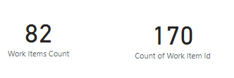
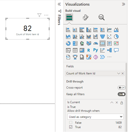
To get the correct count using a default aggregation, you apply the filter Is Current equals 'True.' This pattern of applying filters to a default aggregation is the basis for many of the examples provided in this article.

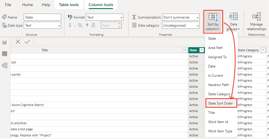
Add State Sort Order

By default, Power BI shows states sorted alphabetically in a visualization. It can be misleading when you want to visualize time in state and Proposed shows up after In Progress. The following steps help to resolve this issue.

1. Verify that the State Category field is included in the Analytics view. This field is included in all default shared views.

2. Select the data table, and then from the Table tools tab, Calculations section of the ribbon, choose New column.

   

3. Replace the default text with the following code and then select the checkmark.

   State Sort Order =  
   SWITCH (  
       'View Name'[State Category],  
       "Proposed", 1,  
       "InProgress", 2,  
       "Resolved", 3,  
       4  
   )  
   

   See the following example:

   

   Note

   You may need to revise the definition if you need more granularity than State Category provides. State Category provides correct sorting across all work item types regardless of any State customizations.

4. Open the Data view and select the State column.

5. From the Column Tools tab, choose Sort by Column and then select the State Sort Order field.

   

Add Date Previous

The next step for calculating time-in-state requires mapping the previous interval (day, week, month) for each row of data in the dataset. It's a simple calculation using a calculated column. Typically, you would define this column as shown.

Date Previous  = 
PREVIOUSDAY ( 'View Name'[Date] )

However, this approach has two main problems:

• It works only for daily periods.
• It doesn't handle gaps in the data. For example, if a work item is moved between projects.

To resolve these problems, the calculated column should find the previous day by scanning the Date field.

To add the Date Previous calculated column, from the Table tools tab, choose New Column and then replace the default text with the following code and select the checkmark.

Date Previous =
CALCULATE (
    MAX ( 'View Name'[Date] ),
        ALLEXCEPT ( 'View Name', 'View Name'[Work Item Id] ),
        'View Name'[Date] < EARLIER ( 'View Name'[Date] )
)

The Date Previous calculated column uses three DAX functions, MAX, ALLEXCEPT, and EARLIER, described in more detail later in this article. Because the column is calculated, it runs for every row in the table, and each time it runs, it has the context of that specific row.

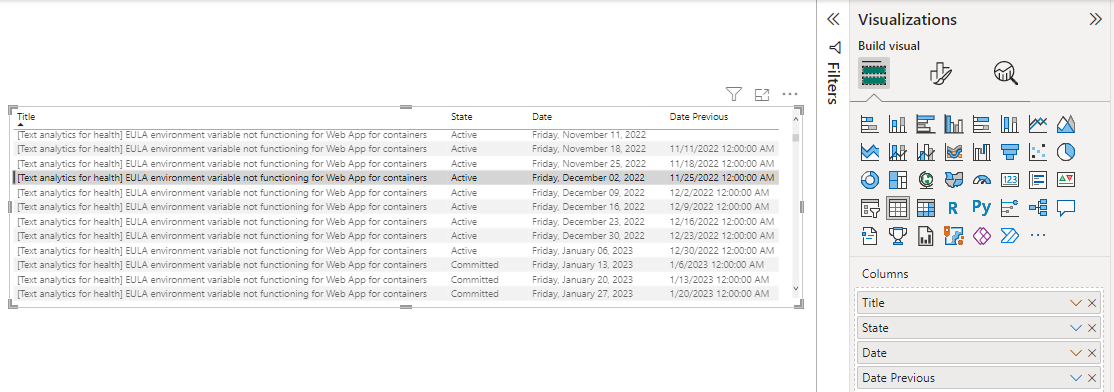
Tip

From the context menu for the Date and Previous Date fields, choose Date (instead of Date Hierarchy) to see a single date for these fields.

Add Date Diff in Days

Date Previous calculates the difference between the previous and current date for each row. With Date Diff in Days, we calculate a count of days between each of those periods. For most rows in a daily snapshot, the value equals 1. However, for many work items that have gaps in the dataset, the value is greater than 1.

Important

Requires that you have added the Date Previous calculated column to the table.

It's important to consider the first day of the dataset where Date Previous is blank. In this example, we give that row a standard value of 1 to keep the calculation consistent.

From the Modeling tab, choose New Column and then replace the default text with the following code and select the checkmark.

Date Diff in Days =
IF (
    ISBLANK ( 'View Name'[Date Previous] ),
    1,
    DATEDIFF (
        'View Name'[Date Previous],
        'View Name'[Date],
        DAY
    )
)

This calculated column uses the ISBLANK and DATEDIFF DAX functions described later in this article.

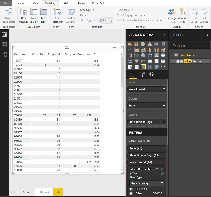
Add Is Last Day in State

In this next step, we calculate if a given row represents the last day a specific work item was in a state. It supports default aggregations in Power BI we add in the next section where we add the State Time in Days column.

From the Modeling tab, choose New Column and then replace the default text with the following code and select the checkmark.

Is Last Day in State = 
ISBLANK (CALCULATE (
    COUNTROWS ( 'View Name' ),
        ALLEXCEPT ( 'View Name', 'View Name'[Work Item Id] ),
        'View Name'[Date] > EARLIER ( 'View Name'[Date] ),
        'View Name'[State] = EARLIER ( 'View Name'[State] )
))

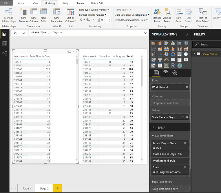
Add State Time in Days

The time that a work item spent in a specific state can now be calculated by summing the Date Diff in Days for each work item. This calculation includes all of the time spent in a specific state even if it switched between states multiple times. It's possible to evaluate each row as a trend using Date or the latest information by using Is Last Day In State.

Important

Requires that you have added the Date Diff in Days and Is Last Day in State calculated columns to the table.

From the Modeling tab, choose New Column and then replace the default text with the following code and select the checkmark.

State Time in Days = 
CALCULATE (
    SUM ( 'View Name'[Date Diff in Days] ),
    ALLEXCEPT ( 'View Name', 'View Name'[Work Item Id] ),
    'View Name'[Date] <= EARLIER ( 'View Name'[Date] ),
    'View Name'[State] = EARLIER ( 'View Name'[State] )
) + 0

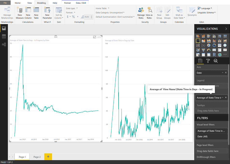
Create stacked column trend charts based on State Time in Days

To demonstrate the State Time in Days column, the following stacked column charts are created. The first chart shows the count of work items in each state over time.

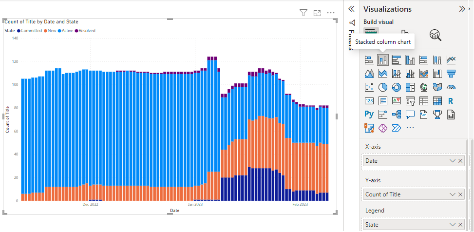
The second chart illustrates the trend of average days the active work items are in a particular state.

Add State Time in Days - Latest (Is Last Day In State)

When evaluating time-in-state for each work item in a table or when filtered by a field like Area Path, don't use the State Time in Days column in an aggregation. The aggregation uses the value for every day the work item was in the state. For example, if a work item was In Progress on Monday and moved to Completed on Thursday, the time-in-state is three days, but the sum of State Time in Days column is six days, 1+2+3, which is incorrect.

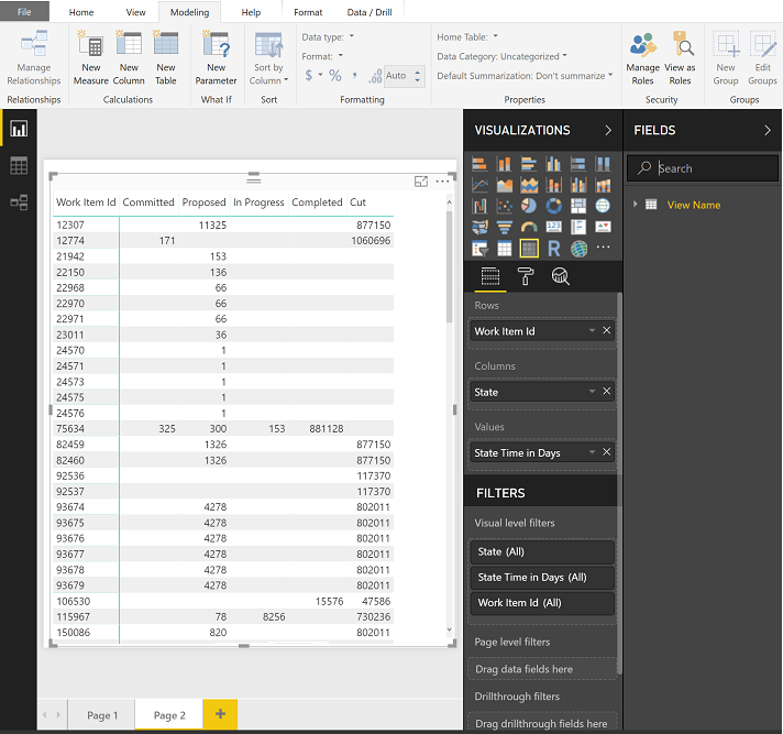
To resolve this issue, use State Time in Days and apply the filter Is Last Day In State equals 'True.' It eliminates all the historical data necessary for a trend and focuses instead on just the latest value for each state.

Add State Time in Days - In Progress

In the previous examples, State Time in Days for a given work item is only counted when the work item was in that specific state. If your goal is to have the time-in-state for a given work item count towards an average continuously, you must change the calculation. For example, if we want to track the "In Progress" state, we add the State Time in Days - In Progress calculated column.

From the Modeling tab, choose New Column and then replace the default text with the following code and select the checkmark.

State Time in Days - In Progress = 
CALCULATE (
    SUM ( 'View Name'[Date Diff in Days] ),
    ALLEXCEPT ( 'View Name', 'View Name'[Work Item Id] ),
   'View Name'[Date] <= EARLIER('View Name'[Date]),
   'View Name'[State] = "In Progress"
) + 0

Note

You may need to revise the definition based on the workflow states used by your project. For example, the project used in the examples in this article use the 'In Progress' workflow state, however, Agile, Scrum, and CMMI processes typically use the 'Active' or 'Committed' states to represent work in progress. For an overview, see Workflow states and state categories.

The following image shows the effect of considering all time-in-state for every existing work item (shown left) versus only those work items in a specific state on a given day (shown right).

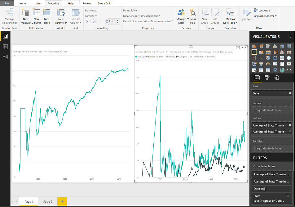
State Time in Days trend of multiple states

Analyzing performance across multiple states is also possible using the "Continuous" pattern. However, this approach only works with a trend chart.

From the Modeling tab, choose New Column and then replace the default text with the following code and select the checkmark.

State Time in Days - Working States = 
CALCULATE (
    SUM ( 'View Name'[Date Diff in Days] ),
    ALLEXCEPT ( 'View Name', 'View Name'[Work Item Id] ),
   'View Name'[Date] <= EARLIER('View Name'[Date]),
   'View Name'[State] IN { "Committed", "In Progress" }
) + 0

Note

You may need to revise the definition based on the workflow states used by your project. For example, if your project uses 'Active' in place of 'Committed' or 'Proposed'.

The chart of the left shows combined average while the right-hand side shows each individual state.

Get the State Time in Days- Latest for multiple states

You use the State Time in Days- Latest calculated column when creating a trend. With a filter on the states, the State Time in Days column and Is Last Day in State provides a simple way to get the total time any work item or group of work items spent in a set of states.

Add State Previous

The Date Previous calculated column can also be used to look up past values such as previous state for each work item.

Important

Requires that you have added the Date Previous calculated column to the table.

From the Modeling tab, choose New Column and then replace the default text with the following code and select the checkmark.

State Previous =
LOOKUPVALUE (
    'View Name'[State],
    'View Name'[Work Item Id], 'View Name'[Work Item Id],
    'View Name'[Date], 'View Name'[Date Previous]
)

This calculated column uses the LOOKUPVALUE, described later in this article.

The first LOOKUPVALUE parameter, 'View Name'[State], specifies to return the value of [State].

The next parameter, 'View Name'[Work Item Id], 'View Name'[Work Item Id], specifies that only rows with a matching work item ID as the current row should be considered.

And, the last parameter, 'View Name'[Date], 'View Name'[Date Previous], specifies that the date of the row being returned must have a [Date] that matches the [Previous Date] of the current row. In a snapshot, only one row can meet this criteria.

Add State Changed

Using the State Previous column, we can flag the rows for each work item where a state transition occurred. The Stage Changed calculated column has two special considerations:

• Blank values of *State Previous, which we set to the Created Date of the work item
• Creation of a work item is considered a state transition

Important

Requires that you have added the State Previous calculated column to the table.

From the Modeling tab, choose New Column and then replace the default text with the following code and select the checkmark.

State Changed =
IF (
    ISBLANK ( 'View Name'[State Previous] ),
    'View Name'[Created Date].[Date] = 'View Name'[Date],
    'View Name'[State Previous] <> 'View Name'[State]
)

The calculated column is a boolean value that identifies whether the row is a state transition. By using the Not Equal To operator, you correctly catch rows where the previous state doesn't match the current state, which means the comparison returns True as expected.

Add State Flow

With State Previous and State Changed calculated columns, you can create a column that illustrates the State Flow for a given work item. Creating this column is optional for the purposes of this article.

Important

Requires that you have added the State Previous and State Changed calculated columns to the table.

From the Modeling tab, choose New Column and then replace the default text with the following code and select the checkmark.

State Flow = 
IF([State Changed], [State Previous], [State]) & " => " & [State]

Add State Change Count

As we move into the more complicated measures, we need to have a representation of the total number of state changes to compare the rows of a data for a given work item. We get the representation by adding a State Change Count calculated column.

Important

Requires that you have added the State Changed calculated column to the table.

From the Modeling tab, choose New Column and then replace the default text with the following code and select the checkmark.

State Change Count = 
CALCULATE (
    COUNTROWS ( 'View Name' ),
    ALLEXCEPT ( 'View Name', 'View Name'[Work Item Id] ),
    'View Name'[Date] <= EARLIER ( 'View Name'[Date] ),
    'View Name'[State Changed]
) + 0

Add State Change Count - Last Proposed and State Restart Time in Days

State Restart Time in Days is a fairly complex calculation. The first step is to find the last time a work item was in a proposed state. Add the State Change Count - Last Proposed calculated column.

Note

You might need to revise the following definitions based on the workflow states used by your project. For example, if your project uses 'New' in place of 'Proposed'.

From the Modeling tab, choose New column and then replace the default text with the following code and select the checkmark.

State Change Count - Last Proposed = 
CALCULATE (
    MAX ( 'View Name'[State Change Count] ),
    ALLEXCEPT ( 'View Name', 'View Name'[Work Item Id] ),
    'View Name'[Date] <= EARLIER ( 'View Name'[Date] ),
    'View Name'[State] = "Proposed"
)

Then, look further back to the past and see if there were some active states before this proposed state. Lastly, sum up all the days when work item was in active state before the last proposed.

From the Modeling tab, choose New Column and then replace the default text with the following code and select the checkmark.

State Restart Time in Days = 
CALCULATE (
    SUM ( 'View Name'[Date Diff in Days] ),
    ALLEXCEPT ( 'View Name', 'View Name'[Work Item Id] ),
    'View Name'[Date] <= EARLIER ( 'View Name'[Date] ),
    'View Name'[State Change Count] < EARLIER('View Name'[State Change Count - Last Proposed] ),
    'View Name'[State] <"Proposed"
) + 0

Since the State Restart Time in Days is updated for each row of data, you can either create a trend to evaluate rework across specific sprints or examine rework for individual work items by using Is Current.

Add State Rework Time in Days

Similar to State Restart Time in Days, the State Rework Time in Days looks for the first time a work item was in the Completed state category. After that time, each day a work item spends in a state other than Completed, counts as rework.

1. Create the "State Change Count - First Completed" column. This column tracks the number of times a work item transitions to the Completed state from any other state.

   State Change Count - First Completed =
   VAR CompletedState = "Completed"
   RETURN
   CALCULATE(
      COUNTROWS('YourTable'),
      FILTER(
          'YourTable',
          'YourTable'[State] = CompletedState
          && 'YourTable'[State Change Date] = MIN('YourTable'[State Change Date])
      )
   )
   

2. From the Modeling tab, choose New Column and then replace the default text with the following code and select the checkmark.

   State Rework Time in Days = 
   IF (
       ISBLANK ( 'View Name'[State Change Count - First Completed] ),
       0,
       CALCULATE (
           SUM ( 'View Name'[Date Diff in Days] ),
           ALLEXCEPT ( 'View Name', 'View Name'[Work Item Id] ),
           'View Name'[Date] <= EARLIER ( 'View Name'[Date] ),
           'View Name'[State Change Count] EARLIER ( 'View Name'[State Change Count - First Completed] ),
           'View Name'[State] IN {"Completed", "Closed", "Cut" } = FALSE()
       ) + 0
   )
   

   Note

   You might need to revise the above definition based on the workflow states used by your project. For example, if your project uses Done in place of Closed, and so on.

DAX functions

Additional information is provided in this section for the DAX functions used to create the calculated columns and measure added in this article. See also DAX, Time intelligence functions.

Function	Description
ALLEXCEPT	Removes all context filters in the table except filters applied to the specified columns. Essentially, ALLEXCEPT ('View Name'', 'View Name'[Work Item Id]) reduces the rows in the table down to only the ones that share the same work item ID as the current row.
CALCULATE	This function is the basis for nearly all examples. The basic structure is an expression followed by a series of filters that are applied to the expression.
COUNTROWS	This function, COUNTROWS ( 'View Name' ), simply counts the number of rows that remain after the filters are applied.
DATEDIFF	Returns the count of interval boundaries crossed between two dates. DATEDIFF subtracts Date Previous from Date to determine the number of days between them.
EARLIER	Returns the current value of the specified column in an outer evaluation pass of the mentioned column. For example, 'View Name'[Date] < EARLIER ( 'View Name'[Date] ) further reduces the data set to only those rows that occurred before the date for the current row that is referenced by using the EARLIER function. EARLIER doesn't refer to previous dates; it specifically defines the row context of the calculated column.
ISBLANK	Checks whether a value is blank, and returns TRUE or FALSE. ISBLANK evaluates the current row to determine if Date Previous has a value. If it doesn't, the If statement sets Date Diff in Days to 1.
LASTDATE	We apply the LASTDATE filter to an expression, for example LASTDATE ( 'View Name'[Date] ), to find the newest date across all rows in the table and eliminate the rows that don't share the same date. With the snapshot table generated by an Analytics view, this filter effectively picks the last day of the selected period.
LOOKUPVALUE	Returns the value in result_columnName for the row that meets all criteria specified by search_columnName and search_value.
MAX	Returns the largest numeric value in a column, or between two scalar expressions. We apply MAX ( 'View Name'[Date] ), to determine the most recent date after all filters are applied.

Related articles

• Power BI integration overview
• Create Analytics views
• Get started with Power BI Desktop
• Dataset design for the Power BI Connector
• Workflow states and state categories
• Data model for Analytics