TartanAir: conjunto de datos de simulación de AirSim para localización y asignación simultáneas (SLAM)
Localización y mapeo simultáneos (SLAM, por sus siglas en inglés) es una de la características más fundamentales necesarias para los robots. Debido a la disponibilidad generalizada de las imágenes, el SLAM visual (V-SLAM) se ha convertido en un componente importante de muchos sistemas autónomos. Se ha conseguido un progreso impresionante tanto con métodos basados en geometría como con métodos basados en el aprendizaje. Sin embargo, el desarrollo de métodos SLAM sólidos y confiables para aplicaciones reales continúa siendo un problema complejo. Los entornos reales están llenos de casos difíciles, como cambios de luz o falta de iluminación, objetos dinámicos y escenas sin texturas. Este conjunto de datos aprovecha los avances de la tecnología de infografía y su objetivo es cubrir diversos escenarios con características de simulación complejas.
Nota
Microsoft proporciona Azure Open Datasets "tal cual". Microsoft no ofrece ninguna garantía, expresa o implícita, ni condición con respecto al uso que usted haga de los conjuntos de datos. En la medida en la que lo permita su legislación local, Microsoft declina toda responsabilidad por posibles daños o pérdidas, incluidos los daños directos, consecuenciales, especiales, indirectos, incidentales o punitivos, que resulten de su uso de los conjuntos de datos.
Este conjunto de datos se proporciona bajo los términos originales con los que Microsoft recibió los datos de origen. El conjunto de datos puede incluir datos procedentes de Microsoft.
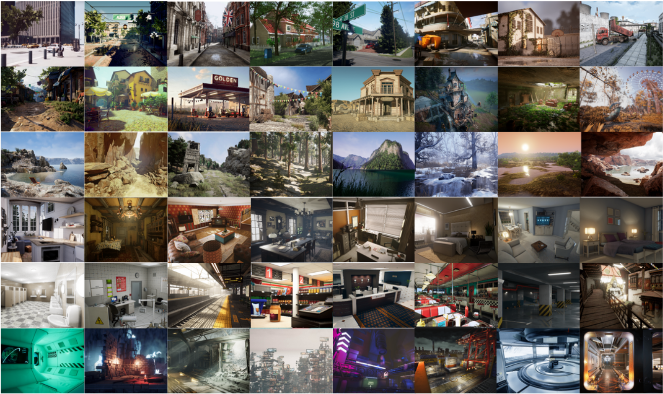
Los datos se recopilan en entornos de simulación fotorrealista con diversas condiciones de iluminación, meteorológicas y de objetos en movimiento. Al recopilar datos de simulaciones, podemos obtener datos de sensor y etiquetas precisas de realidad empírica multimodales, incluidas imágenes RGB estereoscópicas, imágenes con profundidad, segmentación, flujo óptico y posiciones de cámara. Configuramos un gran número de entornos con varios estilos y escenas que cubrían perspectivas difíciles y diversos patrones de movimiento, que son difíciles de lograr usando plataformas de recopilación de datos físicas. Las cuatro características más importantes de nuestro conjunto de datos son: 1) Datos realistas diversos de gran tamaño; 2) Etiquetas de verdad de suelo multimodal; 3) Diversidad de patrones de movimiento; 4) Escenas difíciles.
Este conjunto de datos proporciona cinco tipos de información:
- Imágenes estereoscópicas: tipo imagen (png).
- Archivo de profundidad: tipo numpy (npy).
- Archivo de segmentación: tipo numpy (npy).
- Archivo de flujo óptico: tipo numpy (npy).
- Archivo de posición de cámara: tipo texto (txt).
Los datos se recopilan de diferentes entornos y contienen cientos de trayectorias (3 TB) en total a fecha de 2019.
Efectos visuales complejos
En algunas simulaciones, el conjunto de datos simula varios tipos de efectos visuales complejos.
- Condiciones con mucha luz, alternancia entre día y noche, poca luz y cambios rápidos de iluminación
- Efectos meteorológicos Despejado, lluvia, nieve, viento y niebla
- Cambio estacional
Ubicación de almacenamiento
Este conjunto de datos se almacena en la región Este de EE. UU. de Azure. Se recomienda asignar recursos de proceso de la misma región por afinidad.
Términos de licencia
Este proyecto se publica con la licencia MIT. Revise el archivo de licencia para más detalles.
Información adicional
Consulte el sitio web oficial de TartanAir o el documento de investigación original.
Envíe un correo electrónico a la dirección tartanair@hotmail.com si tiene alguna duda sobre el origen de los datos. También puede ponerse en contacto con los colaboradores en la sección de GitHub asociada.
Notificación Hay más detalles técnicos disponibles en el documento de AirSim (FSR 2017 Conference). Esto se cita del siguiente modo:
@article{tartanair2020arxiv,
  title =   {TartanAir: A Dataset to Push the Limits of Visual SLAM},
  author =  {Wenshan Wang, Delong Zhu, Xiangwei Wang, Yaoyu Hu, Yuheng Qiu, Chen Wang, Yafei Hu, Ashish Kapoor, Sebastian Scherer},
  journal = {arXiv preprint arXiv:2003.14338},
  year =    {2020},
  url = {https://arxiv.org/abs/2003.14338}
}
@inproceedings{airsim2017fsr,
  author = {Shital Shah and Debadeepta Dey and Chris Lovett and Ashish Kapoor},
  title = {AirSim: High-Fidelity Visual and Physical Simulation for Autonomous Vehicles},
  year = {2017},
  booktitle = {Field and Service Robotics},
  eprint = {arXiv:1705.05065},
  url = {https://arxiv.org/abs/1705.05065}
}
Acceso a datos
Use el ejemplo de código siguiente para acceder a los datos de un cuaderno de Python.
Dependencias
pip install numpy
pip install azure-storage-blob
pip install opencv-python
Importación y cliente de contenedor
from azure.storage.blob import ContainerClient
import numpy as np
import io
import cv2
import time
import matplotlib.pyplot as plt
%matplotlib inline

# Dataset website: http://theairlab.org/tartanair-dataset/
account_url = 'https://tartanair.blob.core.windows.net/'
container_name = 'tartanair-release1'

container_client = ContainerClient(account_url=account_url,
                                 container_name=container_name,
                                 credential=None)
Entornos y trayectorias
def get_environment_list():
    '''
    List all the environments shown in the root directory
    '''
    env_gen = container_client.walk_blobs()
    envlist = []
    for env in env_gen:
        envlist.append(env.name)
    return envlist

def get_trajectory_list(envname, easy_hard = 'Easy'):
    '''
    List all the trajectory folders, which is named as 'P0XX'
    '''
    assert(easy_hard=='Easy' or easy_hard=='Hard')
    traj_gen = container_client.walk_blobs(name_starts_with=envname + '/' + easy_hard+'/')
    trajlist = []
    for traj in traj_gen:
        trajname = traj.name
        trajname_split = trajname.split('/')
        trajname_split = [tt for tt in trajname_split if len(tt)>0]
        if trajname_split[-1][0] == 'P':
            trajlist.append(trajname)
    return trajlist

def _list_blobs_in_folder(folder_name):
    """
    List all blobs in a virtual folder in an Azure blob container
    """

    files = []
    generator = container_client.list_blobs(name_starts_with=folder_name)
    for blob in generator:
        files.append(blob.name)
    return files

def get_image_list(trajdir, left_right = 'left'):
    assert(left_right == 'left' or left_right == 'right')
    files = _list_blobs_in_folder(trajdir + '/image_' + left_right + '/')
    files = [fn for fn in files if fn.endswith('.png')]
    return files

def get_depth_list(trajdir, left_right = 'left'):
    assert(left_right == 'left' or left_right == 'right')
    files = _list_blobs_in_folder(trajdir + '/depth_' + left_right + '/')
    files = [fn for fn in files if fn.endswith('.npy')]
    return files

def get_flow_list(trajdir, ):
    files = _list_blobs_in_folder(trajdir + '/flow/')
    files = [fn for fn in files if fn.endswith('flow.npy')]
    return files

def get_flow_mask_list(trajdir, ):
    files = _list_blobs_in_folder(trajdir + '/flow/')
    files = [fn for fn in files if fn.endswith('mask.npy')]
    return files

def get_posefile(trajdir, left_right = 'left'):
    assert(left_right == 'left' or left_right == 'right')
    return trajdir + '/pose_' + left_right + '.txt'

def get_seg_list(trajdir, left_right = 'left'):
    assert(left_right == 'left' or left_right == 'right')
    files = _list_blobs_in_folder(trajdir + '/seg_' + left_right + '/')
    files = [fn for fn in files if fn.endswith('.npy')]
    return files
Enumeración de entornos
envlist = get_environment_list()
print('Find {} environments..'.format(len(envlist)))
print(envlist)
Enumeración de las trayectorias "fáciles" en el primer entorno
diff_level = 'Easy'
env_ind = 0
trajlist = get_trajectory_list(envlist[env_ind], easy_hard = diff_level)
print('Find {} trajectories in {}'.format(len(trajlist), envlist[env_ind]+diff_level))
print(trajlist)
Enumeración de todos los archivos de datos en una sola trayectoria
traj_ind = 1
traj_dir = trajlist[traj_ind]

left_img_list = get_image_list(traj_dir, left_right = 'left')
print('Find {} left images in {}'.format(len(left_img_list), traj_dir))

right_img_list = get_image_list(traj_dir, left_right = 'right')
print('Find {} right images in {}'.format(len(right_img_list), traj_dir))

left_depth_list = get_depth_list(traj_dir, left_right = 'left')
print('Find {} left depth files in {}'.format(len(left_depth_list), traj_dir))

right_depth_list = get_depth_list(traj_dir, left_right = 'right')
print('Find {} right depth files in {}'.format(len(right_depth_list), traj_dir))

left_seg_list = get_seg_list(traj_dir, left_right = 'left')
print('Find {} left segmentation files in {}'.format(len(left_seg_list), traj_dir))

right_seg_list = get_seg_list(traj_dir, left_right = 'left')
print('Find {} right segmentation files in {}'.format(len(right_seg_list), traj_dir))

flow_list = get_flow_list(traj_dir)
print('Find {} flow files in {}'.format(len(flow_list), traj_dir))

flow_mask_list = get_flow_mask_list(traj_dir)
print('Find {} flow mask files in {}'.format(len(flow_mask_list), traj_dir))

left_pose_file = get_posefile(traj_dir, left_right = 'left')
print('Left pose file: {}'.format(left_pose_file))

right_pose_file = get_posefile(traj_dir, left_right = 'right')
print('Right pose file: {}'.format(right_pose_file))
Funciones de descarga de datos
def read_numpy_file(numpy_file,):
    '''
    return a numpy array given the file path
    '''
    bc = container_client.get_blob_client(blob=numpy_file)
    data = bc.download_blob()
    ee = io.BytesIO(data.content_as_bytes())
    ff = np.load(ee)
    return ff


def read_image_file(image_file,):
    '''
    return a uint8 numpy array given the file path
    '''
    bc = container_client.get_blob_client(blob=image_file)
    data = bc.download_blob()
    ee = io.BytesIO(data.content_as_bytes())
    img=cv2.imdecode(np.asarray(bytearray(ee.read()),dtype=np.uint8), cv2.IMREAD_COLOR)
    im_rgb = img[:, :, [2, 1, 0]] # BGR2RGB
    return im_rgb
Introducción a la visualización de datos
def depth2vis(depth, maxthresh = 50):
    depthvis = np.clip(depth,0,maxthresh)
    depthvis = depthvis/maxthresh*255
    depthvis = depthvis.astype(np.uint8)
    depthvis = np.tile(depthvis.reshape(depthvis.shape+(1,)), (1,1,3))

    return depthvis

def seg2vis(segnp):
    colors = [(205, 92, 92), (0, 255, 0), (199, 21, 133), (32, 178, 170), (233, 150, 122), (0, 0, 255), (128, 0, 0), (255, 0, 0), (255, 0, 255), (176, 196, 222), (139, 0, 139), (102, 205, 170), (128, 0, 128), (0, 255, 255), (0, 255, 255), (127, 255, 212), (222, 184, 135), (128, 128, 0), (255, 99, 71), (0, 128, 0), (218, 165, 32), (100, 149, 237), (30, 144, 255), (255, 0, 255), (112, 128, 144), (72, 61, 139), (165, 42, 42), (0, 128, 128), (255, 255, 0), (255, 182, 193), (107, 142, 35), (0, 0, 128), (135, 206, 235), (128, 0, 0), (0, 0, 255), (160, 82, 45), (0, 128, 128), (128, 128, 0), (25, 25, 112), (255, 215, 0), (154, 205, 50), (205, 133, 63), (255, 140, 0), (220, 20, 60), (255, 20, 147), (95, 158, 160), (138, 43, 226), (127, 255, 0), (123, 104, 238), (255, 160, 122), (92, 205, 92),]
    segvis = np.zeros(segnp.shape+(3,), dtype=np.uint8)

    for k in range(256):
        mask = segnp==k
        colorind = k % len(colors)
        if np.sum(mask)>0:
            segvis[mask,:] = colors[colorind]

    return segvis

def _calculate_angle_distance_from_du_dv(du, dv, flagDegree=False):
    a = np.arctan2( dv, du )

    angleShift = np.pi

    if ( True == flagDegree ):
        a = a / np.pi * 180
        angleShift = 180
        # print("Convert angle from radian to degree as demanded by the input file.")

    d = np.sqrt( du * du + dv * dv )

    return a, d, angleShift

def flow2vis(flownp, maxF=500.0, n=8, mask=None, hueMax=179, angShift=0.0):
    """
    Show a optical flow field as the KITTI dataset does.
    Some parts of this function is the transform of the original MATLAB code flow_to_color.m.
    """

    ang, mag, _ = _calculate_angle_distance_from_du_dv( flownp[:, :, 0], flownp[:, :, 1], flagDegree=False )

    # Use Hue, Saturation, Value colour model
    hsv = np.zeros( ( ang.shape[0], ang.shape[1], 3 ) , dtype=np.float32)

    am = ang < 0
    ang[am] = ang[am] + np.pi * 2

    hsv[ :, :, 0 ] = np.remainder( ( ang + angShift ) / (2*np.pi), 1 )
    hsv[ :, :, 1 ] = mag / maxF * n
    hsv[ :, :, 2 ] = (n - hsv[:, :, 1])/n

    hsv[:, :, 0] = np.clip( hsv[:, :, 0], 0, 1 ) * hueMax
    hsv[:, :, 1:3] = np.clip( hsv[:, :, 1:3], 0, 1 ) * 255
    hsv = hsv.astype(np.uint8)

    rgb = cv2.cvtColor(hsv, cv2.COLOR_HSV2RGB)

    if ( mask is not None ):
        mask = mask > 0
        rgb[mask] = np.array([0, 0 ,0], dtype=np.uint8)

    return rgb
Descarga y visualización
data_ind = 173 # randomly select one frame (data_ind < TRAJ_LEN)

left_img = read_image_file(left_img_list[data_ind])
right_img = read_image_file(right_img_list[data_ind])

# Visualize the left and right RGB images
plt.figure(figsize=(12, 5))
plt.subplot(121)
plt.imshow(left_img)
plt.title('Left Image')
plt.subplot(122)
plt.imshow(right_img)
plt.title('Right Image')
plt.show()

# Visualize the left and right depth files
left_depth = read_numpy_file(left_depth_list[data_ind])
left_depth_vis = depth2vis(left_depth)

right_depth = read_numpy_file(right_depth_list[data_ind])
right_depth_vis = depth2vis(right_depth)

plt.figure(figsize=(12, 5))
plt.subplot(121)
plt.imshow(left_depth_vis)
plt.title('Left Depth')
plt.subplot(122)
plt.imshow(right_depth_vis)
plt.title('Right Depth')
plt.show()

# Visualize the left and right segmentation files
left_seg = read_numpy_file(left_seg_list[data_ind])
left_seg_vis = seg2vis(left_seg)

right_seg = read_numpy_file(right_seg_list[data_ind])
right_seg_vis = seg2vis(right_seg)

plt.figure(figsize=(12, 5))
plt.subplot(121)
plt.imshow(left_seg_vis)
plt.title('Left Segmentation')
plt.subplot(122)
plt.imshow(right_seg_vis)
plt.title('Right Segmentation')
plt.show()

# Visualize the flow and mask files

flow = read_numpy_file(flow_list[data_ind])
flow_vis = flow2vis(flow)

flow_mask = read_numpy_file(flow_mask_list[data_ind])
flow_vis_w_mask = flow2vis(flow, mask = flow_mask)

plt.figure(figsize=(12, 5))
plt.subplot(121)
plt.imshow(flow_vis)
plt.title('Optical Flow')
plt.subplot(122)
plt.imshow(flow_vis_w_mask)
plt.title('Optical Flow w/ Mask')
plt.show()
Pasos siguientes
Consulte el resto de los conjuntos de datos en el catálogo de Open Datasets.