Estimating Correlation and Variance/Covariance Matrices
Important
This content is being retired and may not be updated in the future. The support for Machine Learning Server will end on July 1, 2022. For more information, see What's happening to Machine Learning Server?
The rxCovCor function in RevoScaleR calculates the covariance, correlation, or sum of squares/cross-product matrix for a set of variables in a .xdf file or data frame. The size of these matrices is determined by the number of variables rather than the number of observations, so typically the results can easily fit into memory in R. A broad category of analyses can be computed from some form of a cross-product matrix, for example, factor analysis and principal components.
A cross-product matrix is a matrix of the form X'X, where X represents an arbitrary set of raw or standardized variables. More generally, this matrix is of the form X'WX, where W is a diagonal weighting matrix.
Computing Cross-Product Matrices
While rxCovCor is the primary tool for computing covariance, correlation, and other cross-product matrices, you will seldom call it directly. Instead, it is generally simpler to use one of the following convenience functions:
- rxCov: Use rxCov to return the covariance matrix
- rxCor: Use rxCor to return the correlation matrix
- rxSSCP: Use rxSSCP to return the augmented cross-product matrix, that is, we first add a column of 1’s (if no weights are specified) or a column equaling the square root of the weights to the data matrix, and then compute the cross-product.
Computing a Correlation Matrix for Use in Factor Analysis
The 5% sample of the U.S. 2000 census has over 14 million observations. In this example, we compute the correlation matrix for 16 variables derived from variables in the data set for individuals over the age of 20. This correlation matrix is then used as input into the standard R factor analysis function, factanal.
First, we specify the name and location of the data set:
#  Computing a Correlation Matrix for Use in Factor Analysis

bigDataDir <- "C:/MRS/Data"
bigCensusData <- file.path(bigDataDir, "Census5PCT2000.xdf"
Next, we can take a quick look at some basic demographic and socio-economic variables by calling rxSummary. (For more information on variables in the census data, see http://usa.ipums.org/usa-action/variables/group.) Throughout the analysis we use the probability weighting variable, perwt, and restrict the analysis to people over the age of 20.
The
blocksPerReadargument is ignored if run locally using R Client. Learn more...
rxSummary(~phone + speakeng + wkswork1 + incwelfr + incss + educrec + metro +
	ownershd + marst + lingisol + nfams + yrsusa1 + movedin + racwht + age,
	data = bigCensusData, blocksPerRead = 5, pweights = "perwt",
	rowSelection = age > 20)
This call provides summary information about the variables in this weighted subsample, including cell counts for factor variables:
Call:
rxSummary(formula = ~phone + speakeng + wkswork1 + incwelfr +
	incss + educrec + metro + ownershd + marst + lingisol + nfams +
	yrsusa1 + movedin + racwht + age, data = censusData, pweights = "perwt",
	rowSelection = age > 20, blocksPerRead = 5)

Summary Statistics Results for: ~phone + speakeng + wkswork1 + incwelfr
	+ incss + educrec + metro + ownershd + marst + lingisol + nfams +
	yrsusa1 + movedin + racwht + age
File name: C:\MRS\Data\Census5PCT2000.xdf
Probability weights: perwt
Number of valid observations: 9822124

	Name     Mean        StdDev       Min Max   SumOfWeights MissingWeights
	wkswork1   32.068473   23.2438663  0     52 196971131    0
	incwelfr   61.155293  711.0955602  0  25500 196971131    0
	incss    1614.604835 3915.7717233  0  26800 196971131    0
	nfams       1.163434    0.5375238  1     48 196971131    0
	yrsusa1     2.868573    9.0098343  0     90 196971131    0
	age        46.813005   17.1797905 21     93 196971131    0

Category Counts for phone
Number of categories: 3

	phone                  Counts
	N/A                      5611380
	No, no phone available   3957030
	Yes, phone available   187402721

Category Counts for speakeng
Number of categories: 10

	speakeng                 Counts
	N/A (Blank)                      0
	Does not speak English     2956934
	Yes, speaks English...           0
	Yes, speaks only English 162425091
	Yes, speaks very well     17664738
	Yes, speaks well           7713303
	Yes, but not well          6211065
	Unknown                          0
	Illegible                        0
	Blank                            0

Category Counts for educrec
Number of categories: 10

	educrec                 Counts
	N/A  or No schooling           0
	None or preschool        2757363
	Grade 1, 2, 3, or 4      1439820
	Grade 5, 6, 7, or 8     10180870
	Grade 9                  4862980
	Grade 10                 5957922
	Grade 11                 5763456
	Grade 12                63691961
	1 to 3 years of college 55834997
	4+ years of college     46481762

Category Counts for metro
Number of categories: 5

	metro                                Counts
	Not applicable                       13829398
	Not in metro area                    32533836
	In metro area, central city          32080416
	In metro, area, outside central city 60836302
	Central city status unknown          57691179

Category Counts for ownershd
Number of categories: 8

	ownershd                    Counts
	N/A                          5611380
	Owned or being bought              0
	Check mark (owns?)                 0
	Owned free and clear        40546259
	Owned with mortgage or loan 94626060
	Rents                              0
	No cash rent                 3169987
	With cash rent              53017445

Category Counts for marst
Number of categories: 6

	marst                      Counts
	Married, spouse present    112784037
	Married, spouse absent       5896245
	Separated                    4686951
	Divorced                    21474299
	Widowed                     14605829
	Never married/single (N/A)  37523770

Category Counts for lingisol
Number of categories: 3

	lingisol                    Counts
	N/A (group quarters/vacant)   5611380
	Not linguistically isolated 182633786
	Linguistically isolated       8725965

Category Counts for movedin
Number of categories: 7

	movedin                Counts
	NA                     92708540
	This year or last year 20107246
	2-5 years ago          30328210
	6-10 years ago         16959897
	11-20 years ago        16406155
	21-30 years ago        10339278
	31+ years ago          10121805

Category Counts for racwht
Number of categories: 2

	racwht Counts
	No      40684944
	Yes    156286187
Next we call the rxCor function, a convenience function for rxCovCor that returns just the Pearson’s correlation matrix for the variables specified. We make heavy use of the transforms argument to create a series of logical (or dummy) variables from factor variables to be used in the creation of the correlation matrix.
censusCor <- rxCor(formula=~poverty + noPhone + noEnglish  + onSocialSecurity +
	onWelfare + working + incearn + noHighSchool + inCity + renter +
	noSpouse + langIsolated + multFamilies + newArrival + recentMove +
	white + sei + older,
	data = bigCensusData, pweightsb= "perwt", blocksPerRead = 5,
	rowSelection = age > 20,
	transforms= list(
		noPhone = phone == "No, no phone available",
		noEnglish = speakeng == "Does not speak English",
		working = wkswork1 > 20,
		onWelfare = incwelfr > 0,
		onSocialSecurity = incss > 0,
		noHighSchool =
			!(educrec %in%
			c("Grade 12", "1 to 3 years of college", "4+ years of college")),
		inCity = metro == "In metro area, central city",
		renter = ownershd %in% c("No cash rent", "With cash rent"),
		noSpouse = marst != "Married, spouse present",
		langIsolated = lingisol == "Linguistically isolated",
		multFamilies = nfams > 2,
		newArrival = yrsusa2 == "0-5 years",
		recentMove = movedin == "This year or last year",
		white = racwht == "Yes",
		older = age > 64
		))
The resulting correlation matrix is used as input into the factor analysis function provided by the stats package in R. In interpreting the results, the variable poverty represents family income as a percentage of a poverty threshold, so increases as family income increases. First, specify two factors:
censusFa <- factanal(covmat = censusCor, factors=2)
print(censusFa, digits=2, cutoff = .2, sort= TRUE)
Results in:
Call:
factanal(factors = 2, covmat = censusCor)

Uniquenesses:
			poverty          noPhone        noEnglish onSocialSecurity
			0.53             0.96             0.93             0.23
		onWelfare          working          incearn     noHighSchool
			0.96             0.51             0.68             0.82
			inCity           renter         noSpouse     langIsolated
			0.97             0.79             0.90             0.90
	multFamilies       newArrival       recentMove            white
			0.96             0.93             0.97             0.88
				sei            older
			0.57             0.24

Loadings:
					Factor1 Factor2
onSocialSecurity  0.83   -0.29
working          -0.68
sei              -0.59   -0.29
older             0.82   -0.29
poverty          -0.28   -0.63
noPhone
noEnglish                 0.26
onWelfare
incearn          -0.46   -0.34
noHighSchool      0.31    0.29
inCity
renter                    0.45
noSpouse                  0.28
langIsolated              0.31
multFamilies
newArrival                0.26
recentMove
white                    -0.34

				Factor1 Factor2
SS loadings       2.60    1.67
Proportion Var    0.14    0.09
Cumulative Var    0.14    0.24

The degrees of freedom for the model is 118 and the fit was 0.6019
We can use the same correlation matrix to estimate three factors:
censusFa <- factanal(covmat = censusCor, factors=3)
print(censusFa, digits=2, cutoff = .2, sort= TRUE)

	Call:
	factanal(factors = 3, covmat = censusCor)

	Uniquenesses:
			poverty          noPhone        noEnglish onSocialSecurity
				0.49             0.96             0.72             0.24
			onWelfare          working          incearn     noHighSchool
				0.96             0.50             0.62             0.80
			inCity           renter         noSpouse     langIsolated
				0.96             0.80             0.90             0.59
		multFamilies       newArrival       recentMove            white
				0.96             0.79             0.97             0.88
				sei            older
				0.56             0.22

	Loadings:
					Factor1 Factor2 Factor3
	onSocialSecurity  0.87
	working          -0.62    0.34
	sei              -0.51    0.42
	older             0.88
	poverty                   0.68
	incearn          -0.36    0.51
	noEnglish                         0.53
	langIsolated                      0.64
	noPhone
	onWelfare                -0.21
	noHighSchool      0.25   -0.26    0.26
	inCity
	renter                   -0.36    0.24
	noSpouse                 -0.30
	multFamilies
	newArrival                        0.46
	recentMove
	white                     0.24   -0.24

					Factor1 Factor2 Factor3
	SS loadings       2.41    1.50    1.18
	Proportion Var    0.13    0.08    0.07
	Cumulative Var    0.13    0.22    0.28
The degrees of freedom for the model is 102 and the fit was 0.343
Computing A Covariance Matrix for Principal Components Analysis
Principal components analysis, or PCA, is a technique closely related to factor analysis. PCA seeks to find a set of orthogonal axes such that the first axis, or first principal component, accounts for as much variability as possible, and subsequent axes or components are chosen to maximize variance while maintaining orthogonality with previous axes. Principal components are typically computed either by a singular value decomposition of the data matrix or an eigenvalue decomposition of a covariance or correlation matrix; the latter permits us to use rxCovCor and its relatives with the standard R function princomp.
As an example, we use the rxCov function to calculate a covariance matrix for the log of the classic iris data, and pass the matrix to the princomp function (reproduced from Modern Applied Statistics with S):
#  Computing A Covariance Matrix for Principal Components Analysis

irisLog <- as.data.frame(lapply(iris[,1:4], log))
irisSpecies <- iris[,5]
irisCov <- rxCov(~ Sepal.Length + Sepal.Width + Petal.Length + Petal.Width,
	data=irisLog)
irisPca <- princomp(covmat=irisCov, cor=TRUE)
summary(irisPca)
Yields the following:
Importance of components:
							Comp.1    Comp.2     Comp.3    Comp.4
Standard deviation     1.7124583 0.9523797 0.36470294 0.1656840
Proportion of Variance 0.7331284 0.2267568 0.03325206 0.0068628
Cumulative Proportion  0.7331284 0.9598851 0.99313720 1.0000000
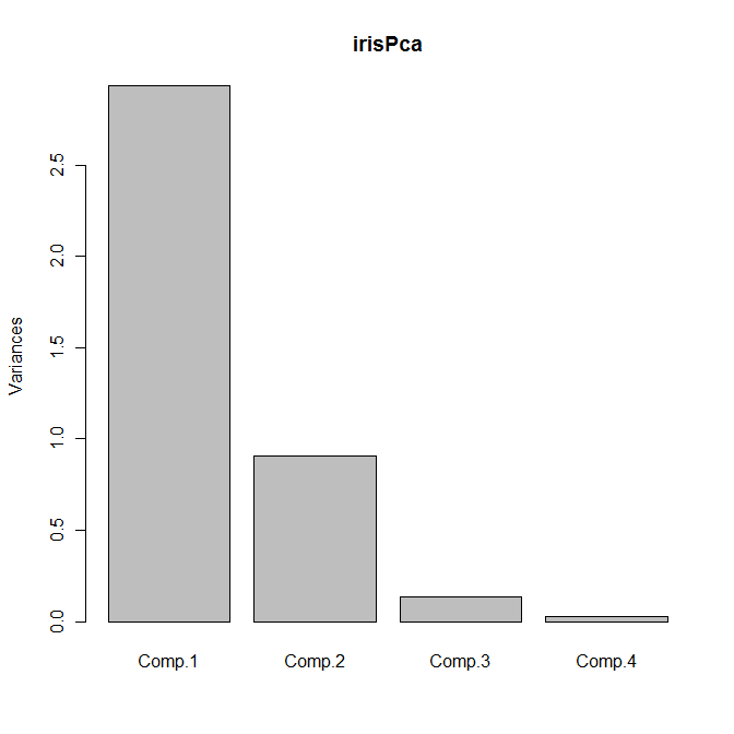
The default plot method for objects of class princomp is a scree plot, which is a barplot of the variances of the principal components. We can obtain the plot as usual by calling plot with our principal components object:
plot(irisPca)
Yields the following plot:
Another useful bit of output is given by the loadings function, which returns a set of columns showing the linear combinations for each principal component:
loadings(irisPca)

	Loadings:
				Comp.1 Comp.2 Comp.3 Comp.4
	Sepal.Length  0.504 -0.455  0.709  0.191
	Sepal.Width  -0.302 -0.889 -0.331
	Petal.Length  0.577        -0.219 -0.786
	Petal.Width   0.567        -0.583  0.580

					Comp.1 Comp.2 Comp.3 Comp.4
	SS loadings      1.00   1.00   1.00   1.00
	Proportion Var   0.25   0.25   0.25   0.25
	Cumulative Var   0.25   0.50   0.75   1.00
You may have noticed that we supplied the flag cor=TRUE in the call to princomp; this flag tells princomp to use the correlation matrix rather than the covariance matrix to compute the principal components. We can obtain the same results by omitting the flag but submitting the correlation matrix as returned by rxCor instead:
irisCor <- rxCor(~ Sepal.Length + Sepal.Width + Petal.Length + Petal.Width,
	data=irisLog)
irisPca2 <- princomp(covmat=irisCor)
summary(irisPca2)
loadings(irisPca2)
plot(irisPca2)
A Large Data Principal Components Analysis
Stock market data for open, high, low, close, and adjusted close from 1962 to 2010 is available at https://github.com/thebigjc/HackReduce/blob/master/datasets/nyse/daily_prices/NYSE_daily_prices_subset.csv. The full data set includes 9.2 million observations of daily open-high-low-close data for some 2800 stocks. As you might expect, these data are highly correlated, and principal components analysis can be used for data reduction. We read the original data into a .xdf file, NYSE_daily_prices.xdf, using the same process we used in the Tutorial: Analyzing loan data with RevoScaleR to read our mortgage data (set revoDataDir to the full path to the NYSE directory containing the .csv files when you unpack the download):
#  A Large Data Principal Components Analysis

if (bHasNYSE){

bigDataDir <- "C:/MRS/Data"
nyseCsvFiles <- file.path(bigDataDir, "NYSE_daily_prices","NYSE",
	"NYSE_daily_prices_")

nyseXdf <- "NYSE_daily_prices.xdf"
append <- "none"
for (i in LETTERS)
{
	importFile <- paste(nyseCsvFiles, i, ".csv", sep="")
	rxImport(importFile, nyseXdf, append=append)
	append <- "rows"
}
Once we have our .xdf file, we proceed as before:
stockCor <- rxCor(~ stock_price_open + stock_price_high +
	stock_price_low + stock_price_close +
	stock_price_adj_close, data="NYSE_daily_prices.xdf")
stockPca <- princomp(covmat=stockCor)
summary(stockPca)
loadings(stockPca)
plot(stockPca)
Yields the following output:
> summary(stockPca)
Importance of components:
							Comp.1    Comp.2      Comp.3       Comp.4
Standard deviation     2.0756631 0.8063270 0.197632281 0.0454173922
Proportion of Variance 0.8616755 0.1300327 0.007811704 0.0004125479
Cumulative Proportion  0.8616755 0.9917081 0.999519853 0.9999324005
								Comp.5
Standard deviation     1.838470e-02
Proportion of Variance 6.759946e-05
Cumulative Proportion  1.000000e+00
> loadings(stockPca)

Loadings:
						Comp.1 Comp.2 Comp.3 Comp.4 Comp.5
stock_price_open      -0.470 -0.166  0.867
stock_price_high      -0.477 -0.151 -0.276  0.410 -0.711
stock_price_low       -0.477 -0.153 -0.282  0.417  0.704
stock_price_close     -0.477 -0.149 -0.305 -0.811
stock_price_adj_close -0.309  0.951

				Comp.1 Comp.2 Comp.3 Comp.4 Comp.5
SS loadings       1.0    1.0    1.0    1.0    1.0
Proportion Var    0.2    0.2    0.2    0.2    0.2
Cumulative Var    0.2    0.4    0.6    0.8    1.0
The scree plot is shown as follows:
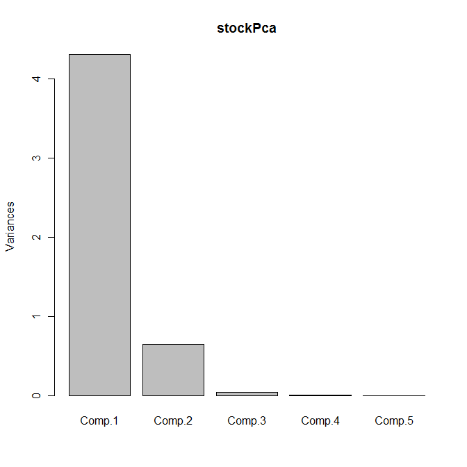
Between them, the first two principal components explain 99% of the variance; we can therefore replace the five original variables by these two principal components with no appreciable loss of information.
Ridge Regression
Another application of correlation matrices is to calculate ridge regression, a type of regression that can help deal with multicollinearity and is part of a broader class of models called Penalized Regression Models.
Where the ordinary least squares regression minimizes the sum of squared residuals

ridge regression minimizes the slightly modified sum
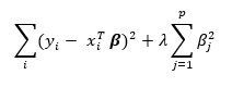
The solution to the ridge regression is

where  is the model matrix. This matrix is similar to the ordinary least squares regression solution with a “ridge” added along the diagonal.
Since the model matrix is embedded in the correlation matrix, the following function allows us to compute the ridge regression solution:
#  Ridge regression
rxRidgeReg <- function(formula, data, lambda, ...) {
  myTerms <- all.vars(formula)
  newForm <- as.formula(paste("~", paste(myTerms, collapse = "+")))
  myCor <- rxCovCor(newForm, data = data, type = "Cor", ...)
  n <- myCor$valid.obs
  k <- nrow(myCor$CovCor) - 1
  bridgeprime <- do.call(rbind, lapply(lambda,
        function(l) qr.solve(myCor$CovCor[-1,-1] + l*diag(k),
                             myCor$CovCor[-1,1])))
  bridge <-  myCor$StdDevs[1] * sweep(bridgeprime, 2,
        myCor$StdDevs[-1], "/")
  bridge <- cbind(t(myCor$Means[1] -
        tcrossprod(myCor$Means[-1], bridge)), bridge)
  rownames(bridge) <- format(lambda)
  return(bridge)
}
The following example shows how ridge regression dramatically improves the solution in a regression involving heavy multicollinearity:
set.seed(14)
x <- rnorm(100)
y <- rnorm(100, mean=x, sd=.01)
z <- rnorm(100, mean=2 + x +y)
data <- data.frame(x=x, y=y, z=z)
lm(z ~ x + y)

 Call:
 lm(formula = z ~ x + y)

 Coefficients:
 (Intercept)            x            y
	  1.827        4.359       -2.584
rxRidgeReg(z ~ x + y, data=data, lambda=0.02)
					  x         y
 0.02 1.827674 0.8917924 0.8723334
You can supply a vector of lambdas as a quick way to compare various choices:
rxRidgeReg(z ~ x + y, data=data, lambda=c(0, 0.02, 0.2, 2, 20))
                        x           y
  0.00 1.827112 4.35917238 -2.58387778
  0.02 1.827674 0.89179239  0.87233344
  0.20 1.833899 0.81020130  0.80959911
  2.00 1.865339 0.44512940  0.44575060
 20.00 1.896779 0.08092296  0.08105322
For λ = 0, the ridge regression is identical to ordinary least squares, while as λ → ∞, the coefficients of x and y approach 0.