TartanAir: 동시 지역화 및 매핑을 위한 AirSim 시뮬레이션 데이터 세트(SLAM)
SLAM(Simultaneous Localization and Mapping)은 로봇에 필요한 가장 기본적인 기능 중 하나입니다. 이미지를 어디서나 사용할 수 있어 V-SLAM(시각적 SLAM)은 많은 자치 시스템의 중요한 구성 요소가 되었습니다. 기하 기반 메서드와 학습 기반 메서드 모두에서 인상적인 발전이 이루어졌습니다. 그러나 실제 애플리케이션을 위한 강력하고 안정적인 SLAM 메서드를 개발하는 것은 여전히 어려운 문제입니다. 실제 환경은 빛의 변화 또는 조명 부족, 동적 개체 및 질감 없는 장면 등 어려운 경우로 가득합니다. 이 데이터 세트는 발전하는 컴퓨터 그래픽 기술을 활용하고 시뮬레이션에서 어려운 기능으로 다양한 시나리오를 다루는 것을 목표로 합니다.
참고 항목
Microsoft는 Azure Open Datasets를 “있는 그대로” 제공합니다. Microsoft는 귀하의 데이터 세트 사용과 관련하여 어떠한 명시적이거나 묵시적인 보증, 보장 또는 조건을 제공하지 않습니다. 귀하가 거주하는 지역의 법규가 허용하는 범위 내에서 Microsoft는 귀하의 데이터 세트 사용으로 인해 발생하는 일체의 직접적, 결과적, 특별, 간접적, 부수적 또는 징벌적 손해 또는 손실을 비롯한 모든 손해 또는 손실에 대한 모든 책임을 부인합니다.
이 데이터 세트는 Microsoft가 원본 데이터를 받은 원래 사용 약관에 따라 제공됩니다. 데이터 세트에는 Microsoft가 제공한 데이터가 포함될 수 있습니다.
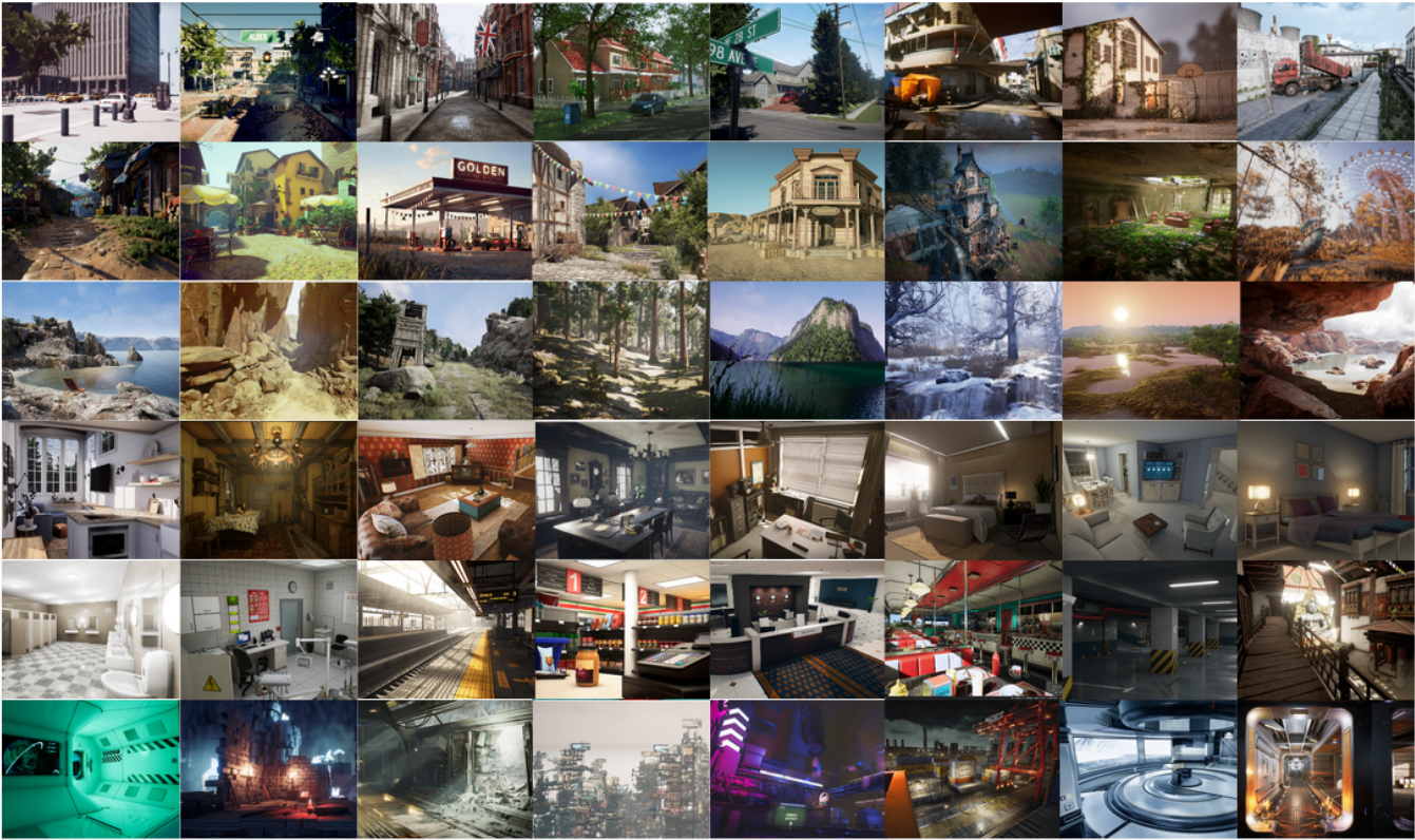
이 데이터는 다양한 빛 조건, 날씨 및 움직이는 개체가 있는 사실적 시뮬레이션 환경에서 수집됩니다. 시뮬레이션에서 데이터를 수집하여 스테레오 RGB 이미지, 깊이 이미지, 세그먼트화, 광학 흐름, 카메라 포즈 등 다중 모달 센서 데이터 및 정밀한 지상 실측 레이블을 얻을 수 있습니다. 다양한 스타일과 장면으로 많은 환경을 설정하여 물리적 데이터 수집 플랫폼을 사용해서는 달성하기 어려운 도전적인 뷰포인트와 다양한 모션 패턴을 다룹니다. 데이터 세트의 가장 중요한 네 가지 기능은 1) 다양한 대규모 실제 데이터, 2) 다중 모달 지상 실측 레이블, 3) 동작 패턴의 다양성, 4) 어려운 장면입니다.
이 데이터 세트는 다음과 같은 5가지 형식의 데이터를 제공합니다.
- 스테레오 이미지: 이미지 형식(PNG)
- 깊이 파일: numpy 형식(NPY)
- 세그먼트화 파일: numpy 형식(NPY)
- 광학 흐름 파일: numpy 형식(NPY)
- 카메라 포즈 파일: 텍스트 형식(TXT)
다양한 환경에서 수집되었으며, 2019년 기준으로 총 수백 개의 궤도(3TB)를 포함합니다.
어려운 시각적 효과
어떤 시뮬레이션에서는 해당 데이터 세트가 여러 유형의 어려운 시각적 효과를 시뮬레이션합니다.
- 강한 빛 조건 낮과 밤의 반복 약한 빛 빠르게 변화하는 조명
- 날씨 효과 맑음, 비, 눈, 바람 및 안개
- 계절의 변화
스토리지 위치
이 데이터 세트는 미국 동부 Azure 지역에 저장됩니다. 선호도를 위해 미국 동부에 컴퓨팅 리소스를 할당하는 것이 좋습니다.
사용 조건
이 프로젝트는 MIT 라이선스에 따라 릴리스되었습니다. 자세한 내용은 라이선스 파일을 검토하세요.
추가 정보
공식적인 TartanAir 웹 사이트를 보거나 원본 연구 논문을 참조하세요.
데이터 원본에 대한 질문이 있는 경우 tartanair@hotmail.com로 문의해 주세요. 관련 GitHub에서 기여자에게 문의할 수도 있습니다.
인용 추가 기술 세부 정보는 AirSim 논문(FSR 2017 컨퍼런스)에서에서 확인할 수 있습니다. 다음과 같이 인용합니다.
@article{tartanair2020arxiv,
  title =   {TartanAir: A Dataset to Push the Limits of Visual SLAM},
  author =  {Wenshan Wang, Delong Zhu, Xiangwei Wang, Yaoyu Hu, Yuheng Qiu, Chen Wang, Yafei Hu, Ashish Kapoor, Sebastian Scherer},
  journal = {arXiv preprint arXiv:2003.14338},
  year =    {2020},
  url = {https://arxiv.org/abs/2003.14338}
}
@inproceedings{airsim2017fsr,
  author = {Shital Shah and Debadeepta Dey and Chris Lovett and Ashish Kapoor},
  title = {AirSim: High-Fidelity Visual and Physical Simulation for Autonomous Vehicles},
  year = {2017},
  booktitle = {Field and Service Robotics},
  eprint = {arXiv:1705.05065},
  url = {https://arxiv.org/abs/1705.05065}
}
데이터 액세스
다음 코드 샘플을 사용하여 Python Notebook의 데이터에 액세스합니다.
종속성
pip install numpy
pip install azure-storage-blob
pip install opencv-python
가져오기 및 컨테이너 클라이언트
from azure.storage.blob import ContainerClient
import numpy as np
import io
import cv2
import time
import matplotlib.pyplot as plt
%matplotlib inline

# Dataset website: http://theairlab.org/tartanair-dataset/
account_url = 'https://tartanair.blob.core.windows.net/'
container_name = 'tartanair-release1'

container_client = ContainerClient(account_url=account_url,
                                 container_name=container_name,
                                 credential=None)
환경 및 궤도
def get_environment_list():
    '''
    List all the environments shown in the root directory
    '''
    env_gen = container_client.walk_blobs()
    envlist = []
    for env in env_gen:
        envlist.append(env.name)
    return envlist

def get_trajectory_list(envname, easy_hard = 'Easy'):
    '''
    List all the trajectory folders, which is named as 'P0XX'
    '''
    assert(easy_hard=='Easy' or easy_hard=='Hard')
    traj_gen = container_client.walk_blobs(name_starts_with=envname + '/' + easy_hard+'/')
    trajlist = []
    for traj in traj_gen:
        trajname = traj.name
        trajname_split = trajname.split('/')
        trajname_split = [tt for tt in trajname_split if len(tt)>0]
        if trajname_split[-1][0] == 'P':
            trajlist.append(trajname)
    return trajlist

def _list_blobs_in_folder(folder_name):
    """
    List all blobs in a virtual folder in an Azure blob container
    """

    files = []
    generator = container_client.list_blobs(name_starts_with=folder_name)
    for blob in generator:
        files.append(blob.name)
    return files

def get_image_list(trajdir, left_right = 'left'):
    assert(left_right == 'left' or left_right == 'right')
    files = _list_blobs_in_folder(trajdir + '/image_' + left_right + '/')
    files = [fn for fn in files if fn.endswith('.png')]
    return files

def get_depth_list(trajdir, left_right = 'left'):
    assert(left_right == 'left' or left_right == 'right')
    files = _list_blobs_in_folder(trajdir + '/depth_' + left_right + '/')
    files = [fn for fn in files if fn.endswith('.npy')]
    return files

def get_flow_list(trajdir, ):
    files = _list_blobs_in_folder(trajdir + '/flow/')
    files = [fn for fn in files if fn.endswith('flow.npy')]
    return files

def get_flow_mask_list(trajdir, ):
    files = _list_blobs_in_folder(trajdir + '/flow/')
    files = [fn for fn in files if fn.endswith('mask.npy')]
    return files

def get_posefile(trajdir, left_right = 'left'):
    assert(left_right == 'left' or left_right == 'right')
    return trajdir + '/pose_' + left_right + '.txt'

def get_seg_list(trajdir, left_right = 'left'):
    assert(left_right == 'left' or left_right == 'right')
    files = _list_blobs_in_folder(trajdir + '/seg_' + left_right + '/')
    files = [fn for fn in files if fn.endswith('.npy')]
    return files
환경 나열
envlist = get_environment_list()
print('Find {} environments..'.format(len(envlist)))
print(envlist)
첫 번째 환경의 '간편' 궤도 나열
diff_level = 'Easy'
env_ind = 0
trajlist = get_trajectory_list(envlist[env_ind], easy_hard = diff_level)
print('Find {} trajectories in {}'.format(len(trajlist), envlist[env_ind]+diff_level))
print(trajlist)
모든 데이터 파일을 하나의 궤도에 나열
traj_ind = 1
traj_dir = trajlist[traj_ind]

left_img_list = get_image_list(traj_dir, left_right = 'left')
print('Find {} left images in {}'.format(len(left_img_list), traj_dir))

right_img_list = get_image_list(traj_dir, left_right = 'right')
print('Find {} right images in {}'.format(len(right_img_list), traj_dir))

left_depth_list = get_depth_list(traj_dir, left_right = 'left')
print('Find {} left depth files in {}'.format(len(left_depth_list), traj_dir))

right_depth_list = get_depth_list(traj_dir, left_right = 'right')
print('Find {} right depth files in {}'.format(len(right_depth_list), traj_dir))

left_seg_list = get_seg_list(traj_dir, left_right = 'left')
print('Find {} left segmentation files in {}'.format(len(left_seg_list), traj_dir))

right_seg_list = get_seg_list(traj_dir, left_right = 'left')
print('Find {} right segmentation files in {}'.format(len(right_seg_list), traj_dir))

flow_list = get_flow_list(traj_dir)
print('Find {} flow files in {}'.format(len(flow_list), traj_dir))

flow_mask_list = get_flow_mask_list(traj_dir)
print('Find {} flow mask files in {}'.format(len(flow_mask_list), traj_dir))

left_pose_file = get_posefile(traj_dir, left_right = 'left')
print('Left pose file: {}'.format(left_pose_file))

right_pose_file = get_posefile(traj_dir, left_right = 'right')
print('Right pose file: {}'.format(right_pose_file))
데이터 다운로드 함수
def read_numpy_file(numpy_file,):
    '''
    return a numpy array given the file path
    '''
    bc = container_client.get_blob_client(blob=numpy_file)
    data = bc.download_blob()
    ee = io.BytesIO(data.content_as_bytes())
    ff = np.load(ee)
    return ff


def read_image_file(image_file,):
    '''
    return a uint8 numpy array given the file path
    '''
    bc = container_client.get_blob_client(blob=image_file)
    data = bc.download_blob()
    ee = io.BytesIO(data.content_as_bytes())
    img=cv2.imdecode(np.asarray(bytearray(ee.read()),dtype=np.uint8), cv2.IMREAD_COLOR)
    im_rgb = img[:, :, [2, 1, 0]] # BGR2RGB
    return im_rgb
데이터 시각화 함수
def depth2vis(depth, maxthresh = 50):
    depthvis = np.clip(depth,0,maxthresh)
    depthvis = depthvis/maxthresh*255
    depthvis = depthvis.astype(np.uint8)
    depthvis = np.tile(depthvis.reshape(depthvis.shape+(1,)), (1,1,3))

    return depthvis

def seg2vis(segnp):
    colors = [(205, 92, 92), (0, 255, 0), (199, 21, 133), (32, 178, 170), (233, 150, 122), (0, 0, 255), (128, 0, 0), (255, 0, 0), (255, 0, 255), (176, 196, 222), (139, 0, 139), (102, 205, 170), (128, 0, 128), (0, 255, 255), (0, 255, 255), (127, 255, 212), (222, 184, 135), (128, 128, 0), (255, 99, 71), (0, 128, 0), (218, 165, 32), (100, 149, 237), (30, 144, 255), (255, 0, 255), (112, 128, 144), (72, 61, 139), (165, 42, 42), (0, 128, 128), (255, 255, 0), (255, 182, 193), (107, 142, 35), (0, 0, 128), (135, 206, 235), (128, 0, 0), (0, 0, 255), (160, 82, 45), (0, 128, 128), (128, 128, 0), (25, 25, 112), (255, 215, 0), (154, 205, 50), (205, 133, 63), (255, 140, 0), (220, 20, 60), (255, 20, 147), (95, 158, 160), (138, 43, 226), (127, 255, 0), (123, 104, 238), (255, 160, 122), (92, 205, 92),]
    segvis = np.zeros(segnp.shape+(3,), dtype=np.uint8)

    for k in range(256):
        mask = segnp==k
        colorind = k % len(colors)
        if np.sum(mask)>0:
            segvis[mask,:] = colors[colorind]

    return segvis

def _calculate_angle_distance_from_du_dv(du, dv, flagDegree=False):
    a = np.arctan2( dv, du )

    angleShift = np.pi

    if ( True == flagDegree ):
        a = a / np.pi * 180
        angleShift = 180
        # print("Convert angle from radian to degree as demanded by the input file.")

    d = np.sqrt( du * du + dv * dv )

    return a, d, angleShift

def flow2vis(flownp, maxF=500.0, n=8, mask=None, hueMax=179, angShift=0.0):
    """
    Show a optical flow field as the KITTI dataset does.
    Some parts of this function is the transform of the original MATLAB code flow_to_color.m.
    """

    ang, mag, _ = _calculate_angle_distance_from_du_dv( flownp[:, :, 0], flownp[:, :, 1], flagDegree=False )

    # Use Hue, Saturation, Value colour model
    hsv = np.zeros( ( ang.shape[0], ang.shape[1], 3 ) , dtype=np.float32)

    am = ang < 0
    ang[am] = ang[am] + np.pi * 2

    hsv[ :, :, 0 ] = np.remainder( ( ang + angShift ) / (2*np.pi), 1 )
    hsv[ :, :, 1 ] = mag / maxF * n
    hsv[ :, :, 2 ] = (n - hsv[:, :, 1])/n

    hsv[:, :, 0] = np.clip( hsv[:, :, 0], 0, 1 ) * hueMax
    hsv[:, :, 1:3] = np.clip( hsv[:, :, 1:3], 0, 1 ) * 255
    hsv = hsv.astype(np.uint8)

    rgb = cv2.cvtColor(hsv, cv2.COLOR_HSV2RGB)

    if ( mask is not None ):
        mask = mask > 0
        rgb[mask] = np.array([0, 0 ,0], dtype=np.uint8)

    return rgb
다운로드 및 시각화
data_ind = 173 # randomly select one frame (data_ind < TRAJ_LEN)

left_img = read_image_file(left_img_list[data_ind])
right_img = read_image_file(right_img_list[data_ind])

# Visualize the left and right RGB images
plt.figure(figsize=(12, 5))
plt.subplot(121)
plt.imshow(left_img)
plt.title('Left Image')
plt.subplot(122)
plt.imshow(right_img)
plt.title('Right Image')
plt.show()

# Visualize the left and right depth files
left_depth = read_numpy_file(left_depth_list[data_ind])
left_depth_vis = depth2vis(left_depth)

right_depth = read_numpy_file(right_depth_list[data_ind])
right_depth_vis = depth2vis(right_depth)

plt.figure(figsize=(12, 5))
plt.subplot(121)
plt.imshow(left_depth_vis)
plt.title('Left Depth')
plt.subplot(122)
plt.imshow(right_depth_vis)
plt.title('Right Depth')
plt.show()

# Visualize the left and right segmentation files
left_seg = read_numpy_file(left_seg_list[data_ind])
left_seg_vis = seg2vis(left_seg)

right_seg = read_numpy_file(right_seg_list[data_ind])
right_seg_vis = seg2vis(right_seg)

plt.figure(figsize=(12, 5))
plt.subplot(121)
plt.imshow(left_seg_vis)
plt.title('Left Segmentation')
plt.subplot(122)
plt.imshow(right_seg_vis)
plt.title('Right Segmentation')
plt.show()

# Visualize the flow and mask files

flow = read_numpy_file(flow_list[data_ind])
flow_vis = flow2vis(flow)

flow_mask = read_numpy_file(flow_mask_list[data_ind])
flow_vis_w_mask = flow2vis(flow, mask = flow_mask)

plt.figure(figsize=(12, 5))
plt.subplot(121)
plt.imshow(flow_vis)
plt.title('Optical Flow')
plt.subplot(122)
plt.imshow(flow_vis_w_mask)
plt.title('Optical Flow w/ Mask')
plt.show()
다음 단계
Open Datasets 카탈로그에서 나머지 데이터 세트를 봅니다.