TartanAir: zestaw danych symulacji AirSim na potrzeby jednoczesnej lokalizacji i mapowania (SLAM)
Jednoczesne lokalizowanie i mapowanie (SLAM, Simultaneous Localization and Mapping) to jedna z najbardziej fundamentalnych funkcji niezbędnych dla robotów. Ze względu na powszechną dostępność obrazów wizualne metody SLAM (V-SLAM) stały się ważnym składnikiem wielu systemów autonomicznych. Imponującego postępu dokonano zarówno w przypadku metod geometrycznych, jak i tych opartych na uczeniu. Jednak opracowanie niezawodnych metod SLAM dla rzeczywistych zastosowań nadal stanowi wyzwanie. Rzeczywiste środowiska obfitują w trudne przypadki, takie jak zmiany światła lub jego brak, dynamiczne obiekty oraz sceny bez wyraźnej faktury. Ten zestaw danych wykorzystuje rozwijającą się technologię grafiki komputerowej. Jego celem jest obsłużenie różnych scenariuszy z wymagającymi warunkami w ramach symulacji.
Uwaga
Firma Microsoft udostępnia zestawy danych Platformy Azure open na zasadzie "jak to jest". Firma Microsoft nie udziela żadnych gwarancji, wyraźnych ani domniemanych, gwarancji ani warunków dotyczących korzystania z zestawów danych. W zakresie dozwolonym zgodnie z prawem lokalnym firma Microsoft nie ponosi odpowiedzialności za wszelkie szkody lub straty, w tym bezpośrednie, wynikowe, specjalne, pośrednie, przypadkowe lub karne wynikające z korzystania z zestawów danych.
Zestaw danych jest udostępniany zgodnie z pierwotnymi warunkami, na jakich firma Microsoft otrzymała dane źródłowe. Zestaw danych może zawierać dane pozyskane z firmy Microsoft.
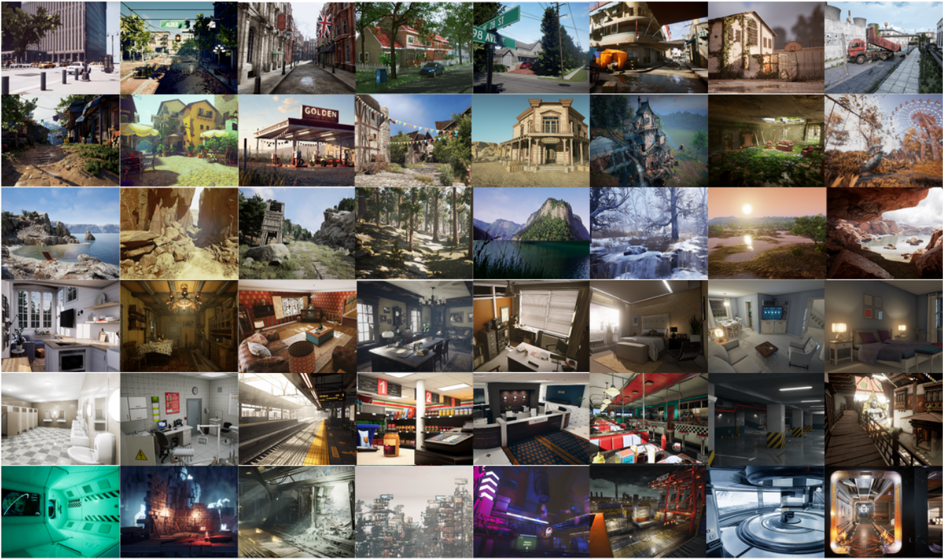
Dane są zbierane w środowiskach symulacji fotorealistycznej w obecności różnych warunków świetlnych, pogody i ruchomych obiektów. Dzięki zbieraniu danych w symulacji możemy uzyskać dane z czujników w wielu trybach i precyzyjne etykiety podstawowych pomiarów, w tym obraz stereo RGB, obraz głębi, segmentację, przepływ optyczny i pozy kamery. Skonfigurowaliśmy dużą liczbę środowisk z różnymi stylami i scenami obejmujących wymagające perspektywy i różnorodne wzorce ruchu, które niełatwo osiągnąć przy użyciu fizycznych platform zbierania danych. Cztery najważniejsze funkcje naszego zestawu danych to: 1) Zróżnicowane realistyczne dane o dużym rozmiarze; 2) Wielomodalne etykiety prawdy podstawowej; 3) Różnorodność wzorców ruchu; 4) Trudne sceny.
Ten zestaw danych zawiera pięć typów danych:
- Obrazy stereo: typ obrazu (PNG)
- Plik głębokości: typ numpy (NPY)
- Plik segmentacji: typ numpy (NPY)
- Plik przepływu optycznego: typ numpy (NPY)
- Plik pozowy aparatu: typ tekstu (TXT)
Jest on zbierany z różnych środowisk, zawiera setki trajektorii (3 TB) w sumie od 2019 roku.
Wymagające efekty wizualne
W niektórych symulacjach zestaw danych symuluje wiele typów wymagających efektów wizualnych.
- Trudne warunki oświetleniowe. Na przemian dzień i noc. Słabe oświetlenie. Szybka zmiana oświetlenia.
- Efekty pogodowe. Bezchmurnie, pada deszcz, pada śnieg, wietrznie i mgła.
- Zmiana pory roku.
Lokalizacja magazynu
Ten zestaw danych jest przechowywany w regionie platformy Azure Wschodnie stany USA. Zalecamy przydzielanie zasobów obliczeniowych w regionie Wschodnie stany USA z uwagi na koligację.
Postanowienia licencyjne
Ten projekt jest publikowany na licencji MIT. Aby uzyskać więcej informacji, zapoznaj się z plikiem licencji .
Dodatkowe informacje
Zobacz oficjalną stronę internetową TartanAir lub przejrzyj oryginalną dokumentację badawczą.
Jeśli masz pytania dotyczące tego zestawu danych, napisz wiadomość e-mail na adres tartanair@hotmail.com. Ponadto można skontaktować się ze współautorami w skojarzonym projekcie GitHub.
Cytat Więcej szczegółów technicznych jest dostępnych w dokumencie AirSim (FSR 2017 Conference). Zacytuj to jako:
@article{tartanair2020arxiv,
  title =   {TartanAir: A Dataset to Push the Limits of Visual SLAM},
  author =  {Wenshan Wang, Delong Zhu, Xiangwei Wang, Yaoyu Hu, Yuheng Qiu, Chen Wang, Yafei Hu, Ashish Kapoor, Sebastian Scherer},
  journal = {arXiv preprint arXiv:2003.14338},
  year =    {2020},
  url = {https://arxiv.org/abs/2003.14338}
}
@inproceedings{airsim2017fsr,
  author = {Shital Shah and Debadeepta Dey and Chris Lovett and Ashish Kapoor},
  title = {AirSim: High-Fidelity Visual and Physical Simulation for Autonomous Vehicles},
  year = {2017},
  booktitle = {Field and Service Robotics},
  eprint = {arXiv:1705.05065},
  url = {https://arxiv.org/abs/1705.05065}
}
Dostęp do danych
Użyj poniższego przykładu kodu, aby uzyskać dostęp do danych w notesie języka Python.
Zależności
pip install numpy
pip install azure-storage-blob
pip install opencv-python
Import i klient kontenera
from azure.storage.blob import ContainerClient
import numpy as np
import io
import cv2
import time
import matplotlib.pyplot as plt
%matplotlib inline

# Dataset website: http://theairlab.org/tartanair-dataset/
account_url = 'https://tartanair.blob.core.windows.net/'
container_name = 'tartanair-release1'

container_client = ContainerClient(account_url=account_url,
                                 container_name=container_name,
                                 credential=None)
Środowiska i trajektorie
def get_environment_list():
    '''
    List all the environments shown in the root directory
    '''
    env_gen = container_client.walk_blobs()
    envlist = []
    for env in env_gen:
        envlist.append(env.name)
    return envlist

def get_trajectory_list(envname, easy_hard = 'Easy'):
    '''
    List all the trajectory folders, which is named as 'P0XX'
    '''
    assert(easy_hard=='Easy' or easy_hard=='Hard')
    traj_gen = container_client.walk_blobs(name_starts_with=envname + '/' + easy_hard+'/')
    trajlist = []
    for traj in traj_gen:
        trajname = traj.name
        trajname_split = trajname.split('/')
        trajname_split = [tt for tt in trajname_split if len(tt)>0]
        if trajname_split[-1][0] == 'P':
            trajlist.append(trajname)
    return trajlist

def _list_blobs_in_folder(folder_name):
    """
    List all blobs in a virtual folder in an Azure blob container
    """

    files = []
    generator = container_client.list_blobs(name_starts_with=folder_name)
    for blob in generator:
        files.append(blob.name)
    return files

def get_image_list(trajdir, left_right = 'left'):
    assert(left_right == 'left' or left_right == 'right')
    files = _list_blobs_in_folder(trajdir + '/image_' + left_right + '/')
    files = [fn for fn in files if fn.endswith('.png')]
    return files

def get_depth_list(trajdir, left_right = 'left'):
    assert(left_right == 'left' or left_right == 'right')
    files = _list_blobs_in_folder(trajdir + '/depth_' + left_right + '/')
    files = [fn for fn in files if fn.endswith('.npy')]
    return files

def get_flow_list(trajdir, ):
    files = _list_blobs_in_folder(trajdir + '/flow/')
    files = [fn for fn in files if fn.endswith('flow.npy')]
    return files

def get_flow_mask_list(trajdir, ):
    files = _list_blobs_in_folder(trajdir + '/flow/')
    files = [fn for fn in files if fn.endswith('mask.npy')]
    return files

def get_posefile(trajdir, left_right = 'left'):
    assert(left_right == 'left' or left_right == 'right')
    return trajdir + '/pose_' + left_right + '.txt'

def get_seg_list(trajdir, left_right = 'left'):
    assert(left_right == 'left' or left_right == 'right')
    files = _list_blobs_in_folder(trajdir + '/seg_' + left_right + '/')
    files = [fn for fn in files if fn.endswith('.npy')]
    return files
Wyświetlanie listy środowisk
envlist = get_environment_list()
print('Find {} environments..'.format(len(envlist)))
print(envlist)
Lista trajektorii "Easy" w pierwszym środowisku
diff_level = 'Easy'
env_ind = 0
trajlist = get_trajectory_list(envlist[env_ind], easy_hard = diff_level)
print('Find {} trajectories in {}'.format(len(trajlist), envlist[env_ind]+diff_level))
print(trajlist)
Wyświetlanie listy wszystkich plików danych w jednej trajektorii
traj_ind = 1
traj_dir = trajlist[traj_ind]

left_img_list = get_image_list(traj_dir, left_right = 'left')
print('Find {} left images in {}'.format(len(left_img_list), traj_dir))

right_img_list = get_image_list(traj_dir, left_right = 'right')
print('Find {} right images in {}'.format(len(right_img_list), traj_dir))

left_depth_list = get_depth_list(traj_dir, left_right = 'left')
print('Find {} left depth files in {}'.format(len(left_depth_list), traj_dir))

right_depth_list = get_depth_list(traj_dir, left_right = 'right')
print('Find {} right depth files in {}'.format(len(right_depth_list), traj_dir))

left_seg_list = get_seg_list(traj_dir, left_right = 'left')
print('Find {} left segmentation files in {}'.format(len(left_seg_list), traj_dir))

right_seg_list = get_seg_list(traj_dir, left_right = 'left')
print('Find {} right segmentation files in {}'.format(len(right_seg_list), traj_dir))

flow_list = get_flow_list(traj_dir)
print('Find {} flow files in {}'.format(len(flow_list), traj_dir))

flow_mask_list = get_flow_mask_list(traj_dir)
print('Find {} flow mask files in {}'.format(len(flow_mask_list), traj_dir))

left_pose_file = get_posefile(traj_dir, left_right = 'left')
print('Left pose file: {}'.format(left_pose_file))

right_pose_file = get_posefile(traj_dir, left_right = 'right')
print('Right pose file: {}'.format(right_pose_file))
Funkcje pobierania danych
def read_numpy_file(numpy_file,):
    '''
    return a numpy array given the file path
    '''
    bc = container_client.get_blob_client(blob=numpy_file)
    data = bc.download_blob()
    ee = io.BytesIO(data.content_as_bytes())
    ff = np.load(ee)
    return ff


def read_image_file(image_file,):
    '''
    return a uint8 numpy array given the file path
    '''
    bc = container_client.get_blob_client(blob=image_file)
    data = bc.download_blob()
    ee = io.BytesIO(data.content_as_bytes())
    img=cv2.imdecode(np.asarray(bytearray(ee.read()),dtype=np.uint8), cv2.IMREAD_COLOR)
    im_rgb = img[:, :, [2, 1, 0]] # BGR2RGB
    return im_rgb
Funkcje wizualizacji danych
def depth2vis(depth, maxthresh = 50):
    depthvis = np.clip(depth,0,maxthresh)
    depthvis = depthvis/maxthresh*255
    depthvis = depthvis.astype(np.uint8)
    depthvis = np.tile(depthvis.reshape(depthvis.shape+(1,)), (1,1,3))

    return depthvis

def seg2vis(segnp):
    colors = [(205, 92, 92), (0, 255, 0), (199, 21, 133), (32, 178, 170), (233, 150, 122), (0, 0, 255), (128, 0, 0), (255, 0, 0), (255, 0, 255), (176, 196, 222), (139, 0, 139), (102, 205, 170), (128, 0, 128), (0, 255, 255), (0, 255, 255), (127, 255, 212), (222, 184, 135), (128, 128, 0), (255, 99, 71), (0, 128, 0), (218, 165, 32), (100, 149, 237), (30, 144, 255), (255, 0, 255), (112, 128, 144), (72, 61, 139), (165, 42, 42), (0, 128, 128), (255, 255, 0), (255, 182, 193), (107, 142, 35), (0, 0, 128), (135, 206, 235), (128, 0, 0), (0, 0, 255), (160, 82, 45), (0, 128, 128), (128, 128, 0), (25, 25, 112), (255, 215, 0), (154, 205, 50), (205, 133, 63), (255, 140, 0), (220, 20, 60), (255, 20, 147), (95, 158, 160), (138, 43, 226), (127, 255, 0), (123, 104, 238), (255, 160, 122), (92, 205, 92),]
    segvis = np.zeros(segnp.shape+(3,), dtype=np.uint8)

    for k in range(256):
        mask = segnp==k
        colorind = k % len(colors)
        if np.sum(mask)>0:
            segvis[mask,:] = colors[colorind]

    return segvis

def _calculate_angle_distance_from_du_dv(du, dv, flagDegree=False):
    a = np.arctan2( dv, du )

    angleShift = np.pi

    if ( True == flagDegree ):
        a = a / np.pi * 180
        angleShift = 180
        # print("Convert angle from radian to degree as demanded by the input file.")

    d = np.sqrt( du * du + dv * dv )

    return a, d, angleShift

def flow2vis(flownp, maxF=500.0, n=8, mask=None, hueMax=179, angShift=0.0):
    """
    Show a optical flow field as the KITTI dataset does.
    Some parts of this function is the transform of the original MATLAB code flow_to_color.m.
    """

    ang, mag, _ = _calculate_angle_distance_from_du_dv( flownp[:, :, 0], flownp[:, :, 1], flagDegree=False )

    # Use Hue, Saturation, Value colour model
    hsv = np.zeros( ( ang.shape[0], ang.shape[1], 3 ) , dtype=np.float32)

    am = ang < 0
    ang[am] = ang[am] + np.pi * 2

    hsv[ :, :, 0 ] = np.remainder( ( ang + angShift ) / (2*np.pi), 1 )
    hsv[ :, :, 1 ] = mag / maxF * n
    hsv[ :, :, 2 ] = (n - hsv[:, :, 1])/n

    hsv[:, :, 0] = np.clip( hsv[:, :, 0], 0, 1 ) * hueMax
    hsv[:, :, 1:3] = np.clip( hsv[:, :, 1:3], 0, 1 ) * 255
    hsv = hsv.astype(np.uint8)

    rgb = cv2.cvtColor(hsv, cv2.COLOR_HSV2RGB)

    if ( mask is not None ):
        mask = mask > 0
        rgb[mask] = np.array([0, 0 ,0], dtype=np.uint8)

    return rgb
Pobieranie i wizualizowanie
data_ind = 173 # randomly select one frame (data_ind < TRAJ_LEN)

left_img = read_image_file(left_img_list[data_ind])
right_img = read_image_file(right_img_list[data_ind])

# Visualize the left and right RGB images
plt.figure(figsize=(12, 5))
plt.subplot(121)
plt.imshow(left_img)
plt.title('Left Image')
plt.subplot(122)
plt.imshow(right_img)
plt.title('Right Image')
plt.show()

# Visualize the left and right depth files
left_depth = read_numpy_file(left_depth_list[data_ind])
left_depth_vis = depth2vis(left_depth)

right_depth = read_numpy_file(right_depth_list[data_ind])
right_depth_vis = depth2vis(right_depth)

plt.figure(figsize=(12, 5))
plt.subplot(121)
plt.imshow(left_depth_vis)
plt.title('Left Depth')
plt.subplot(122)
plt.imshow(right_depth_vis)
plt.title('Right Depth')
plt.show()

# Visualize the left and right segmentation files
left_seg = read_numpy_file(left_seg_list[data_ind])
left_seg_vis = seg2vis(left_seg)

right_seg = read_numpy_file(right_seg_list[data_ind])
right_seg_vis = seg2vis(right_seg)

plt.figure(figsize=(12, 5))
plt.subplot(121)
plt.imshow(left_seg_vis)
plt.title('Left Segmentation')
plt.subplot(122)
plt.imshow(right_seg_vis)
plt.title('Right Segmentation')
plt.show()

# Visualize the flow and mask files

flow = read_numpy_file(flow_list[data_ind])
flow_vis = flow2vis(flow)

flow_mask = read_numpy_file(flow_mask_list[data_ind])
flow_vis_w_mask = flow2vis(flow, mask = flow_mask)

plt.figure(figsize=(12, 5))
plt.subplot(121)
plt.imshow(flow_vis)
plt.title('Optical Flow')
plt.subplot(122)
plt.imshow(flow_vis_w_mask)
plt.title('Optical Flow w/ Mask')
plt.show()
Następne kroki
Wyświetl resztę zestawów danych w katalogu Open Datasets (Otwarte zestawy danych).