Basic R commands and RevoScaleR functions: 25 common examples
Important
This content is being retired and may not be updated in the future. The support for Machine Learning Server will end on July 1, 2022. For more information, see What's happening to Machine Learning Server?
Applies to: Microsoft R Client, Machine Learning Server
If you are new to both R and Machine Learning Server, this tutorial introduces you to 25 (or so) commonly used R functions. In this tutorial, you learn how to load small data sets into R and perform simple computations. A key point to take away from this tutorial is that you can combine basic R commands and RevoScaleR functions in the same R script.
This tutorial starts with R commands before transitioning to RevoScaleR functions. If you already know R, skip ahead to Explore RevoScaleR Functions.
Note
R Client and Machine Learning Server are interchangeable in terms of RevoScaleR as long as data fits into memory and processing is single-threaded. If data size exceeds memory, we recommend pushing the compute context to Machine Learning Server.
Prerequisites
This is our simplest tutorial in terms of data and tools, but it's also expansive in its coverage of basic R and RevoScaleR functions. To complete the tasks, use the command-line tool RGui.exe on Windows or start the Revo64 program on Linux.
- On Windows, go to \Program Files\Microsoft\R Client\R_SERVER\bin\x64 and double-click Rgui.exe.
- On Linux, at the command prompt, type Revo64.
The tutorial uses pre-installed sample data so once you have the software, there is nothing more to download or install.
The R command prompt is >. You can hand-type commands line by line, or copy-paste a multi-line command sequence.
R is case-sensitive. If you hand-type commands in this example, be sure to use the correct case. Windows users: the file paths in R take a forward slash delimiter (/), required even when the path is on the Windows file system.
Start with R
Because RevoScaleR is built on R, this tutorial begins with an exploration of common R commands.
Load data
R is an environment for analyzing data, so the natural starting point is to load some data. For small data sets, such as the following 20 measurements of the speed of light taken from the famous Michelson-Morley experiment, the simplest approach uses R’s c function to combine the data into a vector.
Type or copy the following script and paste it at the > prompt at the beginning of the command line:
c(850, 740, 900, 1070, 930, 850, 950, 980, 980, 880, 1000, 980, 930, 650, 760, 810, 1000, 1000, 960, 960)
When you type the closing parenthesis and press Enter, R responds as follows:
[1]  850  740  900 1070  930  850  950  	980  980  880
[11]  1000 980  930  650  760  810 1000 1000  960  960
This indicates that R has interpreted what you typed, created a vector with 20 elements, and returned that vector. But we have a problem. R hasn’t saved what we typed. If we want to use this vector again (and that’s the usual reason for creating a vector in the first place), we need to assign it. The R assignment operator has the suggestive form <- to indicate a value is being assigned to a name. You can use most combinations of letters, numbers, and periods to form names (but note that names can’t begin with a number). Here we’ll use michelson:
michelson <- c(850, 740, 900, 1070, 930, 850, 950, 980, 980, 880,
1000, 980, 930, 650, 760, 810, 1000, 1000, 960, 960)
R responds with a > prompt. Notice that the named vector is not automatically printed when it is assigned. However, you can view the vector by typing its name at the prompt:
> michelson
Output:
[1]  850  740  900 1070  930  850  950  980   980  880
[11] 1000  980  930  650  760  810 1000 1000  960  960
The c function is useful for hand typing in small vectors such as you might find in textbook examples, and it is also useful for combining existing vectors. For example, if we discovered another five observations that extended the Michelson-Morley data, we could extend the vector using c as follows:
michelsonNew <- c(michelson, 850, 930, 940, 970, 870)
michelsonNew
Output:
[1]  850  740  900 1070  930  850  950  	980  980  880
[11] 1000  980  930  650  760  810 1000 1000  960  960
[21]  850  930  940  970  870
Generate random data
Often for testing purposes you want to use randomly generated data. R has a number of built-in distributions from which you can generate random numbers; two of the most commonly used are the normal and the uniform distributions. To obtain a set of numbers from a normal distribution, you use the rnorm function. This example generates 25 random numbers in a normal distribution.
normalDat <- rnorm(25)
normalDat
Output:
[1] -0.66184983  1.71895416  2.12166699
[4]  1.49715368 -0.03614058  1.23194518
[7] -0.06488077  1.06899373 -0.37696531
[10]  1.04318309 -0.38282188  0.29942160
[13]  0.67423976 -0.29281632  0.48805336
[16]  0.88280182  1.86274898  1.61172529
[19]  0.13547954  1.08808601 -1.26681476
[22] -0.19858329  0.13886578 -0.27933600
[25]  0.70891942
By default, the data are generated from a standard normal with mean 0 and standard deviation 1. You can use the mean and sd arguments to rnorm to specify a different normal distribution:
normalSat <- rnorm(25, mean=450, sd=100)
normalSat
Output:
[1] 373.3390 594.3363 534.4879 410.0630 307.2232
[6] 307.8008 417.1772 478.4570 521.9336 493.2416
[11] 414.8075 479.7721 423.8568 580.8690 451.5870
[16] 406.8826 488.2447 454.1125 444.0776 320.3576
[21] 236.3024 360.6385 511.2733 508.2971 449.4118
Similarly, you can use the runif function to generate random data from a uniform distribution:
uniformDat <- runif(25)
uniformDat
Output:
[1] 0.03105927 0.18295065 0.96637386 0.71535963
[5] 0.16081450 0.15216891 0.07346868 0.15047337
[9] 0.49408599 0.35582231 0.70424152 0.63671421
[13] 0.20865305 0.20167994 0.37511929 0.54082887
[17] 0.86681824 0.23792988 0.44364083 0.88482396
[21] 0.41863803 0.42392873 0.24800036 0.22084038
[25] 0.48285406
Generate a numeric sequence
The default uniform distribution is over the interval 0 to 1. You can specify alternatives by setting the min and max arguments:
uniformPerc <- runif(25, min=0, max=100)
uniformPerc
Output:
[1] 66.221400 12.270863 33.417174 21.985229
[5] 92.767213 17.911602  1.935963 53.551991
[9] 75.110760 22.436347 63.172258 95.977501
[13] 79.317351 56.767608 89.416080 79.546495
[17]  8.961152 49.315612 43.432128 68.871867
[21] 73.598221 63.888835 35.261694 54.481692
[25] 37.575176
Another commonly used vector is the sequence, a uniformly spaced run of numbers. For the common case of a run of integers, you can use the infix operator, :, as follows:
1:10
Output:
[1] 1 2 3 4 5 6 7 8 9 10
For more general sequences, use the seq function:
seq(length = 11, from = 10, to = 30)
Output:
[1] 10 12 14 16 18 20 22 24 26 28 30

seq(from = 10,length = 20, by = 4)
Output:
[1] 10 14 18 22 26 30 34 38 42 46 50 54 58 62 66 70 74
[18] 78 82 86
Tip
If you are working with big data, you’ll still use vectors to manipulate parameters and information about your data, but you'll probably store the data in the RevoScaleR high-performance .xdf file format.
Exploratory Data Analysis
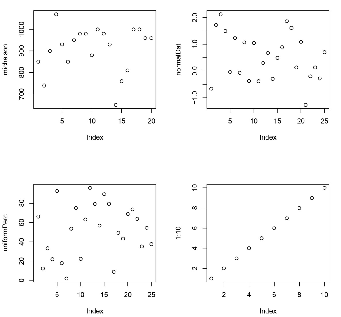
After you have some data, you will want to explore it graphically. For most small data sets, the place to begin is with the plot function, which provides a default graphical view of the data:
plot(michelson)
plot(normalDat)
plot(uniformPerc)
plot(1:10)
For numeric vectors such as ours, the default view is a scatter plot of the observations against their index, resulting in the following plots:
For an exploration of the shape of the data, the usual tools are stem (to create a stemplot) and hist (to create a histogram):
stem(michelson)
Output:
	 The decimal point is 2 digit(s) to the right of the |
	  6 | 5
	  7 | 46
	  8 | 1558
	  9 | 033566888
	 10 | 0007

	hist(michelson)
The resulting histogram is shown as the left plot following. We can make the histogram look more like the stemplot by specifying the nclass argument to hist:
hist(michelson, nclass=5)
The resulting histogram is shown as the right plot in the figure following.
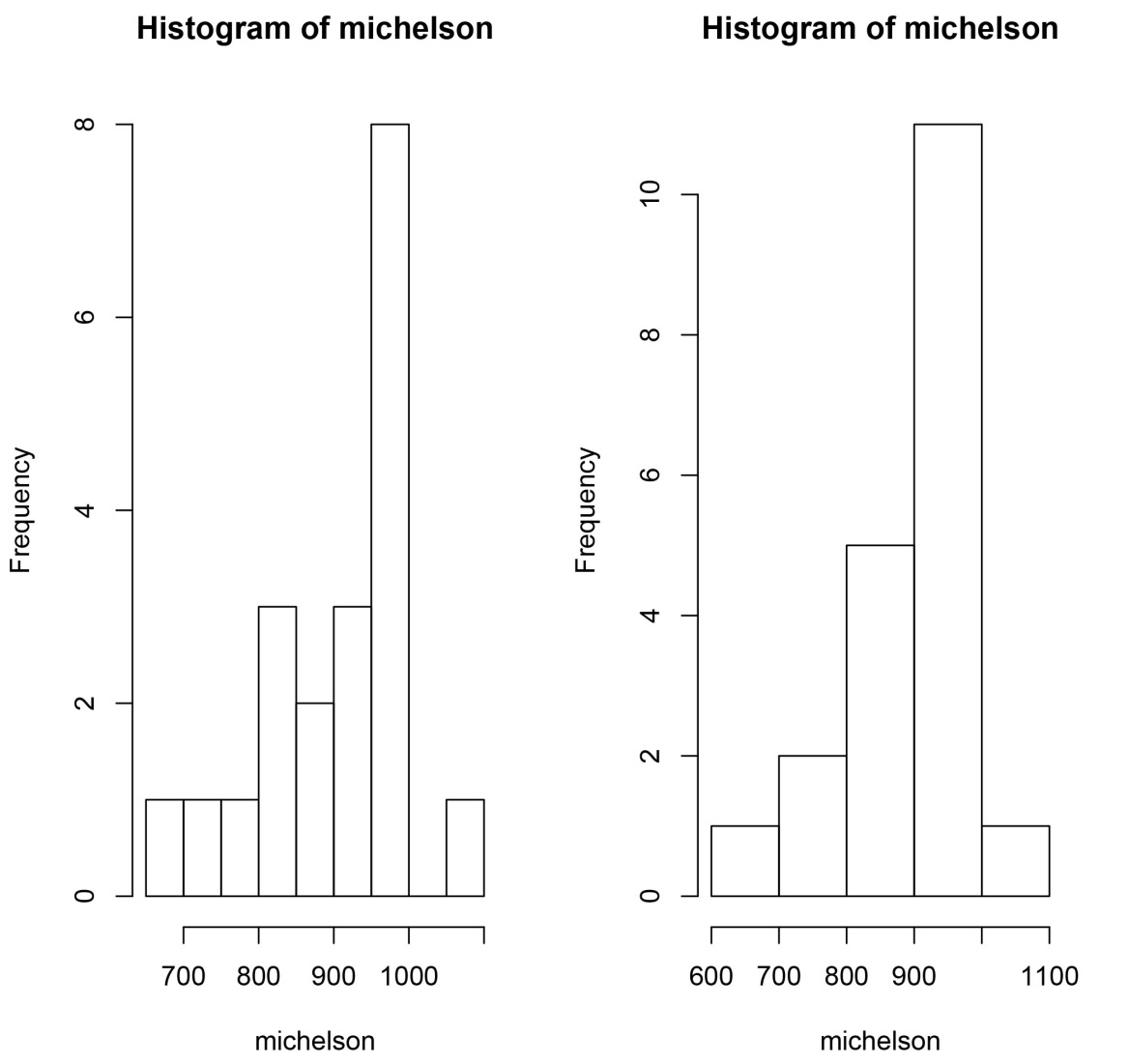
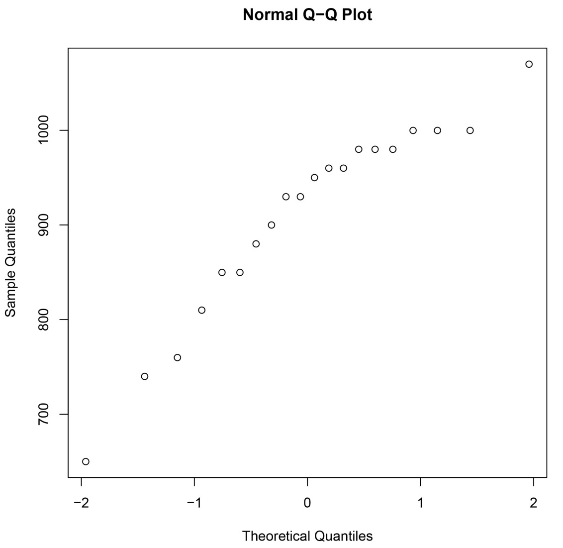
From the histogram and stemplot, it appears that the Michelson-Morley observations are not obviously normal. A normal Q-Q plot gives a graphical test of whether a data set is normal:
qqnorm(michelson)
The decided bend in the resulting plot confirms the suspicion that the data are not normal.
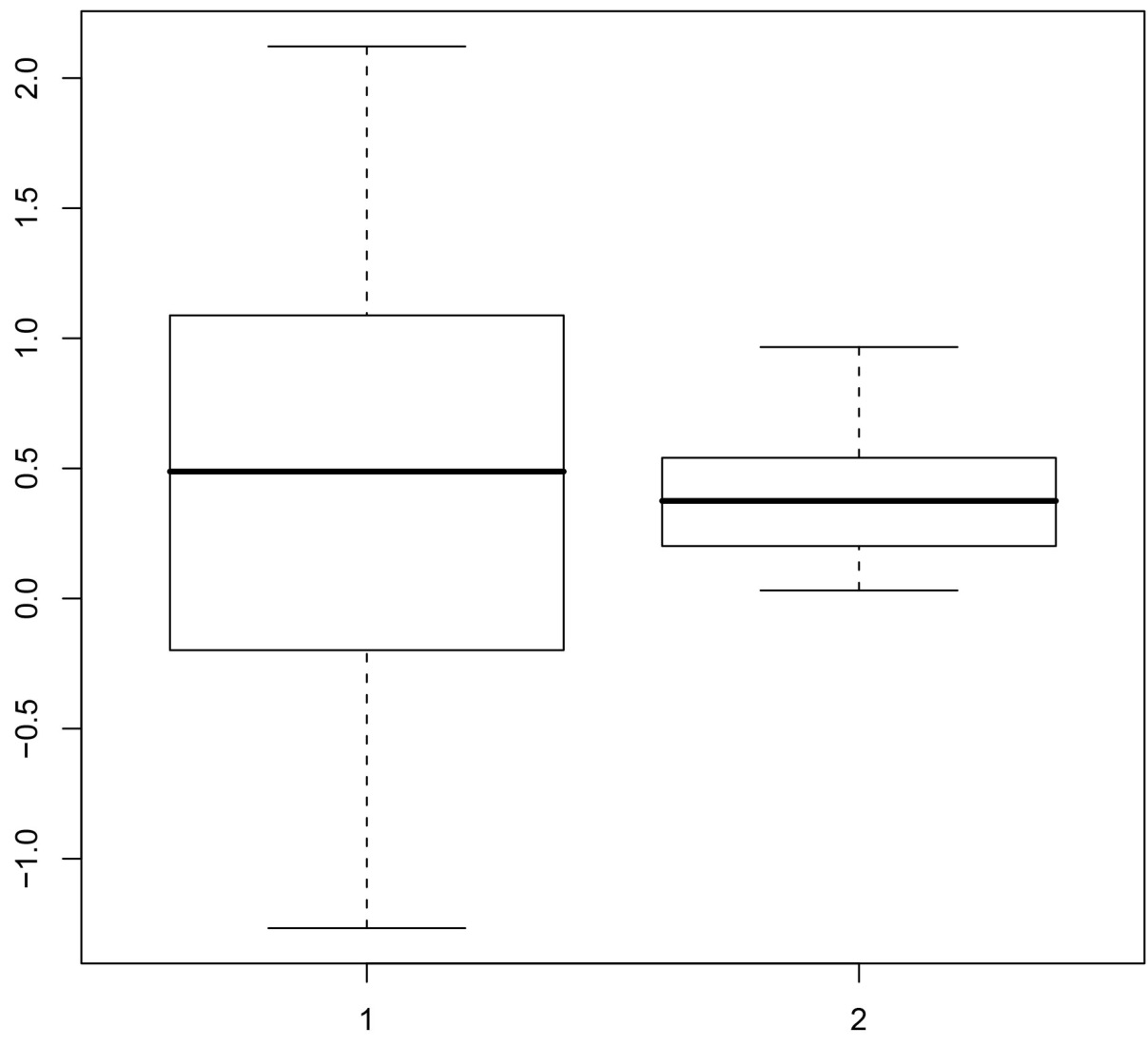
Another useful exploratory plot, especially for comparing two distributions, is the boxplot:
boxplot(normalDat, uniformDat)
Tip
These plots are great if you have a small data set in memory. However, when working with big data, some plot types may not be informative when working directly with the data (for example, scatter plots can produce a large blob of ink) and others may be computational intensive (if sorting is required). A better alternative is the rxHistogram function in RevoScaleR that efficiently computes and renders histograms for large data sets. Additionally, RevoScaleR functions such as rxCube can provide summary information that is easily amenable to the impressive plotting capabilities provided by R packages.
Summary Statistics
While an informative graphic often gives the fullest description of a data set, numerical summaries provide a useful shorthand for describing certain features of the data. For example, estimators such as the mean and median help to locate the data set, and the standard deviation and variance measure the scale or spread of the data. R has a full set of summary statistics available:
> mean(michelson)
[1] 909
> median(michelson)
[1] 940
> sd(michelson)
[1] 104.9260
> var(michelson)
[1] 11009.47
The generic summary function provides a meaningful summary of a data set; for a numeric vector it provides the five-number summary plus the mean:
summary(michelson)
Output:
	 Min. 1st Qu.  Median    Mean 3rd Qu.    Max.
	 650     850     940     909     980    1070
Tip
The rxSummary function in RevoScaleR will efficiently compute summary statistics for a data frame in memory or a large data file stored on disk.
Multivariate Data Sets
In most disciplines, meaningful data sets have multiple variables, typically observations of various quantities and qualities of individual subjects. Such data sets are typically represented as tables in which the columns correspond to variables and the rows correspond to subjects, or cases. In R, such tables can be created as data frame objects. For example, at the 2008 All-Star Break, the Seattle Mariners had five players who met the minimum qualifications to be considered for a batting title (that is, at least 3.1 at bats per game played by the team). Their statistics are shown in the following table:
	Player          Games  AB   R    H   2B  3B   HR   TB  RBI   BA  OBP  SLG  OPS
	"I. Suzuki"        95 391  63  119   11   3    3  145   21 .304 .366 .371 .737
	"J. Lopez"         92 379  46  113   26   1    5  156   48 .298 .318 .412 .729
	"R. Ibanez"        95 370  41  101   26   1   11  162   55 .273 .338 .438 .776
	"Y. Betancourt"    90 326  34   87   22   2    3  122   29 .267 .278 .374 .656
	"A. Beltre"        92 352  46   91   16   0   16  155   46 .259 .329 .440 .769
Copy and paste the table into a text editor (such as Notepad on Windows, or emacs or vi on Unix type machines) and save the file as msStats.txt in the working directory returned by the getwd function, for example:
getwd()
Output:
[1] "/Users/joe"
Tip
On Windows, the working directory is probably a bin folder in program files, and by default you don't have permission to save the file at that location. Use setwd("/Users/TEMP") to change the working directory to /Users/TEMP and save the file.
You can then read the data into R using the read.table function. The argument header=TRUE specifies that the first line is a header of variable names:
msStats <- read.table("msStats.txt", header=TRUE)
msStats
Output:
	Player Games  AB  R   H X2B X3B HR  TB RBI
	1	I. Suzuki     95 391 63 119  11   3  3 145  21
	2	J. Lopez     92 379 46 113  26   1  5 156  48
	3	R. Ibanez     95 370 41 101  26   1 11 162  55
	4 	Y. Betancourt     90 326 34  87  22   2  3 122  29
	5	A. Beltre     92 352 46  91  16   0 16 155  46

		BA   OBP   SLG   OPS
	1 0.304 0.366 0.371 0.737
	2 0.298 0.318 0.412 0.729
	3 0.273 0.338 0.438 0.776
	4 0.267 0.278 0.374 0.656
	5 0.259 0.329 0.440 0.769
Notice how read.table changed the names of our original “2B" and “3B" columns to be valid R names; R names cannot begin with a numeral.
Use built-in datasets package
Most small R data sets in daily use are data frames. The built-in package, datasets, is a rich source of data frames for further experimentation.
To list the data sets in this package, use this command:
ls("package:datasets")
The output is an alphabetized list of data sets that are readily available for use in R functions. In the next section, we will use the built-in data set attitude, available through the datasets package.
Linear Models
The attitude data set is a data frame with 30 observations on 7 variables, measuring the percent proportion of favorable responses to seven survey questions in each of 30 departments. The survey was conducted in a large financial organization; there were approximately 35 respondents in each department.
We mentioned that the plot function could be used with virtually any data set to get an initial visualization; let’s see what it gives for the attitude data:
plot(attitude)
The resulting plot is a pairwise scatter plot of the numeric variables in the data set.
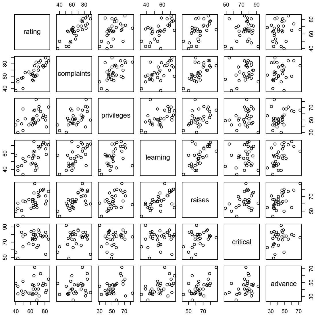
The first two variables (rating and complaints) show a strong linear relationship. To model that relationship, we use the lm function:
attitudeLM1 <- lm(rating ~ complaints, data=attitude)
To view a summary of the model, we can use the summary function:
summary(attitudeLM1)
Output:
	Call:
	lm(formula = rating ~ complaints, data = attitude)
	Residuals:
	   Min       1Q   Median       3Q      Max
	-12.8799  -5.9905   0.1783   6.2978   9.6294

	Coefficients:
		Estimate Std. Error t value Pr(>|t|)
	(Intercept) 14.37632    6.61999   2.172   0.0385 *
	complaints   0.75461    0.09753   7.737 1.99e-08 ***
	---
	Signif. codes:  0 *** 0.001 ** 0.01 * 0.05 . 0.1  1

	Residual standard error: 6.993 on 28 degrees of freedom
	Multiple R-squared: 0.6813, Adjusted R-squared: 0.6699
	F-statistic: 59.86 on 1 and 28 DF,  p-value: 1.988e-08
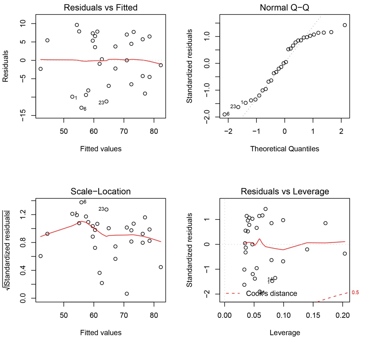
We can also try to visualize the model using plot:
plot(attitudeLM1)
The default plot for a fitted linear model is a set of four plots; by default they are shown one at a time, and you are prompted before each new plot is displayed. To view them all at once, use the par function with the mfrow parameter to specify a 2 x 2 layout:
par(mfrow=c(2,2))
plot(attitudeLM1)
Tip
The rxLinMod function is a full-featured alternative to lm that can efficiently handle large data sets. Also look at rxLogit and rxGlm as alternatives to glm, rxKmeans as an alternative to kmeans, and rxDTree as an alternative to rpart.
Matrices and apply function
A matrix is a two-dimensional data array. Unlike data frames, which can have different data types in their columns, matrices may contain data of only one type. Most commonly, matrices are used to hold numeric data. You create matrices with the matrix function:
A <- matrix(c(3, 5, 7, 9, 13, 15, 8, 4, 2), ncol=3)
A
Output:
[,1] [,2] [,3]
[1,]    3    9    8
[2,]    5   13    4
[3,]    7   15    2
Another matrix example:
B <- matrix(c(4, 7, 9, 5, 8, 6), ncol=3)
B
Output:
[,1] [,2] [,3]
[1,]    4    9    8
[2,]    7    5    6
Ordinary arithmetic acts element-by-element on matrices:
A + A
Output:
[,1] [,2] [,3]
[1,]    6   18   16
[2,]   10   26    8
[3,]   14   30    4
Matrix multiplication uses the expected operators:
A * A
Output:
[,1] [,2] [,3]
[1,]    9   81   64
[2,]   25  169   16
[3,]   49  225    4
Matrix multiplication in the linear algebra sense requires a special operator, %*%:
A %*% A

[,1] [,2] [,3]
[1,]  110  264   76
[2,]  108  274  100
[3,]  110  288  120
Matrix multiplication requires two matrices to be conformable, which means that the number of columns of the first matrix is equal to the number of rows of the second:
B %*% A

[,1] [,2] [,3]
[1,]  113  273   84
[2,]   88  218   88

A %*% B

Error in A %*% B : non-conformable arguments
When you need to manipulate the rows or columns of a matrix, an incredibly useful tool is the apply function. With apply, you can apply a function to all the rows or columns of matrix at once. For example, to find the column products of A, you could use apply as follows:
apply(A, 2, prod)

[1]  105 1755   64
The row products are as simple:
apply(A, 1, prod)

[1] 216 260 210
To sort the columns of A, just replace prod with sort:
	apply(A, 2, sort)

		 [,1] [,2] [,3]
	[1,]    3    9    2
	[2,]    5   13    4
	[3,]    7   15    8
Lists and lapply function
A list in R is a flexible data object that can be used to combine data of different types and different lengths for almost any purpose. Arbitrary lists can be created with either the list function or the c function; many other functions, especially the statistical modeling functions, return their output as list objects.
For example, we can combine a character vector, a numeric vector, and a numeric matrix in a single list as follows:
list1 <- list(x = 1:10, y = c("Tami", "Victor", "Emily"),
z = matrix(c(3, 5, 4, 7), nrow=2))
list1

$x
[1]  1  2  3  4  5  6  7  8  9 10
$y
[1] "Tami"   "Victor" "Emily"
$z
[,1] [,2]
[1,]    3    4
[2,]    5    7
The function lapply can be used to apply the same function to each component of a list in turn:
lapply(list1, length)

$x
[1] 10

$y
[1] 3

$z
[1] 4
Tip
You will regularly use lists and functions that manipulate them when handling input and output for your big data analyses.
Explore RevoScaleR Functions
The RevoScaleR package, included in Machine Learning Server and R Client, provides a framework for quickly writing start-to-finish, scalable R code for data analysis. When you start the R console application on a computer that has Machine Learning Server or R Client, the RevoScaleR function library is loaded automatically.
Load Data with rxImport
The rxImport function allows you to import data from fixed or delimited text files, SAS files, SPSS files, or a SQL Server, Teradata, or ODBC connection. There’s no need to have SAS or SPSS installed on your system to import those file types, but you need a locally installed ODBC driver for your database to access data on a local or remote computer.
Let’s start simply by using a delimited text file available in the built-in sample data directory of the RevoScaleR package. We store the location of the file in a character string (inDataFile), then import the data into an in-memory data set (data frame) called mortData:
inDataFile <- file.path(rxGetOption("sampleDataDir"), "mortDefaultSmall2000.csv")

mortData <- rxImport(inData = inDataFile)
If we anticipate repeating the same analysis on a larger data set later, we could prepare for that by putting placeholders in our code for output files. An output file is an XDF file, native to R Client and Machine Learning Server, persisted on disk and structured to hold modular data. If we included an output file with rxImport, the output object returned from rxImport would be a small object representing the .xdf file on disk (an RxXdfData object), rather than an in-memory data frame containing all of the data.
For now, let's continue to work with the data in memory. We can do this by omitting the outFile argument, or by setting the outFile parameter to NULL. The following code is equivalent to the importing task of that above:
mortOutput <- NULL
mortData <- rxImport(inData = inDataFile, outFile = mortOutput)
Retrieve metadata
There are a number of basic methods we can use to learn about the data set and its variables that work on the return object of rxImport, regardless of whether it is a data frame or RxXdfData object.
To get the number of rows, cols, and names of the imported data:
nrow(mortData)
ncol(mortData)
names(mortData)
Output for these commands is as follows:
> nrow(mortData)
[1] 10000
> ncol(mortData)
[1] 6
> names(mortData)
[1] "creditScore" "houseAge" "yearsEmploy" "ccDebt" "year"
[6] "default"
To print out the first few rows of the data set, you can use head():
head(mortData, n = 3)
Output:
	creditScore houseAge yearsEmploy ccDebt year default
	1 691 16 9 6725 2000 0
	2 691 4 4 5077 2000 0
	3 743 18 3 3080 2000 0
The rxGetInfo function allows you to quickly get information about your data set and its variables all at one time, including more information about variable types and ranges. Let’s try it on mortData, having the first three rows of the data set printed out:
rxGetInfo(mortData, getVarInfo = TRUE, numRows=3)
Output:
Data frame: mortData
Data frame: mortData
Number of observations: 10000
Number of variables: 6
Variable information:
Var 1: creditScore, Type: integer, Low/High: (486, 895)
Var 2: houseAge, Type: integer, Low/High: (0, 40)
Var 3: yearsEmploy, Type: integer, Low/High: (0, 14)
Var 4: ccDebt, Type: integer, Low/High: (0, 12275)
Var 5: year, Type: integer, Low/High: (2000, 2000)
Var 6: default, Type: integer, Low/High: (0, 1)
Data (3 rows starting with row 1):
	creditScore houseAge yearsEmploy ccDebt year default
1 691 16 9 6725 2000 0
2 691 4 4 5077 2000 0
3 743 18 3 3080 2000 0
Select and transform with rxDataStep
The rxDataStep function provides a framework for the majority of your data manipulation tasks. It allows for row selection (the rowSelection argument), variable selection (the varsToKeep or varsToDrop arguments), and the creation of new variables from existing ones (the transforms argument). Here’s an example that does all three with one function call:
outFile2 <- NULL
mortDataNew <- rxDataStep(
	# Specify the input data set
	inData = mortData,
	# Put in a placeholder for an output file
	outFile = outFile2,
	# Specify any variables to keep or drop
	varsToDrop = c("year"),
	# Specify rows to select
	rowSelection = creditScore < 850,
	# Specify a list of new variables to create
	transforms = list(
		catDebt = cut(ccDebt, breaks = c(0, 6500, 13000),
			labels = c("Low Debt", "High Debt")),
		lowScore = creditScore < 625))
Our new data set, mortDataNew, will not have the variable year, but adds two new variables: a categorical variable named catDebt that uses R’s cut function to break the ccDebt variable into two categories, and a logical variable, lowScore, that is TRUE for individuals with low credit scores. These transforms expressions follow the rule that they must be able to operate on a chunk of data at a time; that is, the computation for a single row of data cannot depend on values in other rows of data.
With the rowSelection argument, we have also removed any observations with high credit scores, above or equal to 850. We can use the rxGetVarInfo function to confirm:
rxGetVarInfo(mortDataNew)
Output:
Var 1: creditScore, Type: integer, Low/High: (486, 847)
Var 2: houseAge, Type: integer, Low/High: (0, 40)
Var 3: yearsEmploy, Type: integer, Low/High: (0, 14)
Var 4: ccDebt, Type: integer, Low/High: (0, 12275)
Var 5: default, Type: integer, Low/High: (0, 1)
Var 6: catDebt
	2 factor levels: Low Debt High Debt
Var 7: lowScore, Type: logical, Low/High: (0, 1)
Visualize with rxHistogram, rxCube, and rxLinePlot
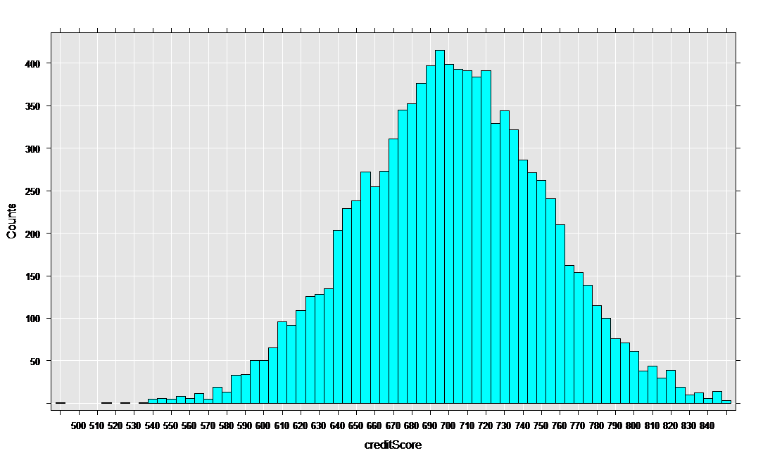
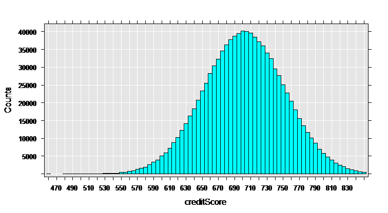
The rxHistogram function shows us the distribution of any of the variables in our data set. For example, let’s look at credit score:
rxHistogram(~creditScore, data = mortDataNew )
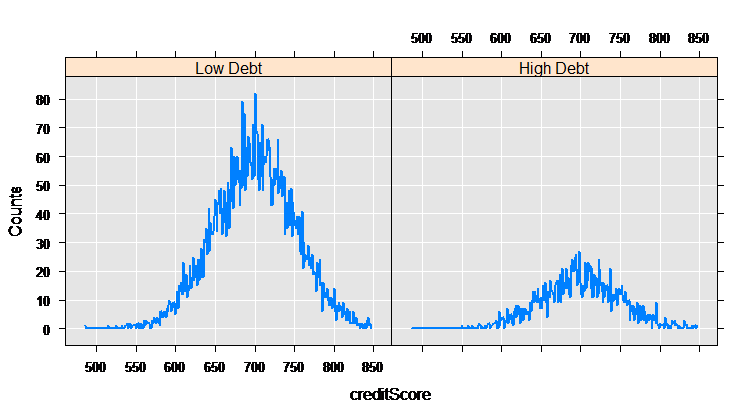
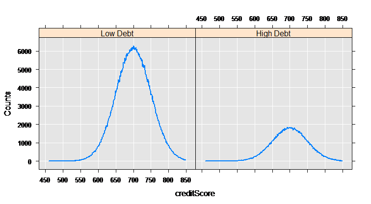
The rxCube function computes category counts, and can operate on the interaction of categorical variables. Using the F() notation to convert a variable into an on-the-fly categorical factor variable (with a level for each integer value), we can compute the counts for each credit score for the two groups who have low and high credit card debt:
mortCube <- rxCube(~F(creditScore):catDebt, data = mortDataNew)
The rxLinePlot function is a convenient way to plot output from rxCube. We use the rxResultsDF helper function to convert cube output into a data frame convenient for plotting:
rxLinePlot(Counts~creditScore|catDebt, data=rxResultsDF(mortCube))
Analyze with rxLogit
RevoScaleR provides the foundation for a variety of high performance, scalable data analyses. Here we do a logistic regression, but you probably also want to take look at computing summary statistics (rxSummary), computing cross-tabs (rxCrossTabs), estimating linear models (rxLinMod) or generalized linear models (rxGlm), and estimating variance-covariance or correlation matrices (rxCovCor) that can be used as inputs to other R functions such as principal components analysis and factor analysis. Now, let’s estimate a logistic regression on whether or not an individual defaulted on their loan, using credit card debt and years of employment as independent variables:
myLogit <- rxLogit(default~ccDebt+yearsEmploy , data=mortDataNew)
summary(myLogit)
We get the following output:
Call:
rxLogit(formula = default ~ ccDebt + yearsEmploy, data = mortDataNew)

Logistic Regression Results for: default ~ ccDebt + yearsEmploy
Data: mortDataNew
Dependent variable(s): default
Total independent variables: 3
Number of valid observations: 9982
Number of missing observations: 0
-2*LogLikelihood: 100.6036 (Residual deviance on 9979 degrees of freedom)

Coefficients:
	Estimate Std. Error z value Pr(>|z|)
(Intercept) -1.614e+01 2.074e+00 -7.781 2.22e-16 ***
ccDebt 1.414e-03 2.139e-04 6.610 3.83e-11 ***
yearsEmploy -3.317e-01 1.608e-01 -2.063 0.0391 *
---
Signif. codes: 0 '***' 0.001 '**' 0.01 '*' 0.05 '.' 0.1 ' ' 1

Condition number of final variance-covariance matrix: 1.4455
Number of iterations: 9
Scale your analysis
Until now, our exploration has been limited to small data sets in memory. Let’s scale up to a data set with a million rows rather than just 10000. These larger text data files are available online. Windows users should download the zip version, mortDefault.zip, and Linux users mortDefault.tar.gz.
After downloading and unpacking the data, set your path to the correct location in the code below. It is more efficient to store the imported data on disk, so we also specify the locations for our imported and transformed data sets:
# bigDataDir <- "C:/MicrosoftR/Data" # Specify the location
inDataFile <- file.path(bigDataDir, "mortDefault",
	"mortDefault2000.csv")
outFile <- "myMortData.xdf"
outFile2 <- "myMortData2.xdf"
That’s it! Now you can reuse all of the importing, data step, plotting, and analysis code preceding on the larger data set.
# Import data
mortData <- rxImport(inData = inDataFile, outFile = outFile)
Output:
Rows Read: 500000, Total Rows Processed: 500000, Total Chunk Time: 1.043 seconds
Rows Read: 500000, Total Rows Processed: 1000000, Total Chunk Time: 1.001 seconds
Because we have specified an output file when importing the data, the returned mortData object is a small object in memory representing the .xdf data file, rather than a full data frame containing all of the data in memory. It can be used in RevoScaleR analysis functions in the same way as data frames.
# Some quick information about my data
rxGetInfo(mortData, getVarInfo = TRUE, numRows=5)
Output:
File name: C:\\MicrosoftR\\Data\\myMortData.xdf
Number of observations: 1e+06
Number of variables: 6
Number of blocks: 2
Compression type: zlib
Variable information:
Var 1: creditScore, Type: integer, Low/High: (459, 942)
Var 2: houseAge, Type: integer, Low/High: (0, 40)
Var 3: yearsEmploy, Type: integer, Low/High: (0, 15)
Var 4: ccDebt, Type: integer, Low/High: (0, 14639)
Var 5: year, Type: integer, Low/High: (2000, 2000)
Var 6: default, Type: integer, Low/High: (0, 1)
Data (5 rows starting with row 1):
creditScore houseAge yearsEmploy ccDebt year default
1 615 10 5 2818 2000 0
2 780 34 5 3575 2000 0
3 735 12 1 3184 2000 0
4 713 15 5 6236 2000 0
5 689 10 5 6817 2000 0
The data step:
mortDataNew <- rxDataStep(
	# Specify the input data set
	inData = mortData,
	# Put in a placeholder for an output file
	outFile = outFile2,
	# Specify any variables to keep or drop
	varsToDrop = c("year"),
	# Specify rows to select
	rowSelection = creditScore < 850,
	# Specify a list of new variables to create
	transforms = list(
		catDebt = cut(ccDebt, breaks = c(0, 6500, 13000),
			labels = c("Low Debt", "High Debt")),
		lowScore = creditScore < 625))
Output:
Rows Read: 500000, Total Rows Processed: 500000, Total Chunk Time: 0.673 seconds
Rows Read: 500000, Total Rows Processed: 1000000, Total Chunk Time: 0.448 seconds
>
Looking at the data:
# Looking at the data
rxHistogram(~creditScore, data = mortDataNew )

	Rows Read: 499294, Total Rows Processed: 499294, Total Chunk Time: 0.329 seconds
	Rows Read: 499293, Total Rows Processed: 998587, Total Chunk Time: 0.335 seconds
	Computation time: 0.678 seconds.
myCube = rxCube(~F(creditScore):catDebt, data = mortDataNew)
rxLinePlot(Counts~creditScore|catDebt, data=rxResultsDF(myCube))
# Compute a logistic regression
myLogit <- rxLogit(default~ccDebt+yearsEmploy , data=mortDataNew)
summary(myLogit)
Output:
Call:
rxLogit(formula = default ~ ccDebt + yearsEmploy, data = mortDataNew)

Logistic Regression Results for: default ~ ccDebt + yearsEmploy
File name:
	C:\Users\RUser\myMortData2.xdf
Dependent variable(s): default
Total independent variables: 3
Number of valid observations: 998587
Number of missing observations: 0
-2*LogLikelihood: 8837.7644 (Residual deviance on 998584 degrees of freedom)

Coefficients:

Estimate Std. Error z value Pr(>|z|)
(Intercept) -1.725e+01 2.330e-01 -74.04 2.22e-16 ***
ccDebt 1.509e-03 2.327e-05 64.85 2.22e-16 ***
yearsEmploy -3.054e-01 1.713e-02 -17.83 2.22e-16 ***
---
Signif. codes: 0 '***' 0.001 '**' 0.01 '*' 0.05 '.' 0.1 ' ' 1

Condition number of final variance-covariance matrix: 1.3005
Number of iterations: 9
Next Steps
Continue on to these tutorials to work with larger data set using the RevoScaleR functions: