Tutorial: Analyzing loan data with RevoScaleR
Important
This content is being retired and may not be updated in the future. The support for Machine Learning Server will end on July 1, 2022. For more information, see What's happening to Machine Learning Server?
This example builds on what you learned in an earlier tutorial by showing you how to import .csv files to create an .xdf file, and use statistical RevoScaleR functions to summarize the data. As before, you'll work with sample data to complete the steps.
Get the mortgage default data set
Data import and exploration are covered further on, but to complete those steps you will need a collection of .csv files providing the sample data.
The sample data used in this tutorial consists of simulated data on mortgage defaults. A small version of the data set is pre-installed with the RevoScaleR package that ships with R Client and Machine Learning Server. It provides 100,000 observations. Alternatively, you can download a larger version of the data set providing 10 million observations.
Use the pre-installed .csv files
Small versions of the data sets can be found in the sample data directory:
mortDefaultSmall2000.csv
mortDefaultSmall2001.csv
mortDefaultSmall2002.csv
mortDefaultSmall2003.csv
mortDefaultSmall2004.csv
mortDefaultSmall2005.csv
mortDefaultSmall2006.csv
mortDefaultSmall2007.csv
mortDefaultSmall2008.csv
mortDefaultSmall2009.csv
Each file contains 10,000 rows, for a total of 100,000 observations.
Download the larger data set
To work with a larger dataset, you can download mortDefault, a set of ten comma-separated files, each of which contains one million observations of simulated data on mortgage defaults. You can download zipped from this web site. Windows users should download the zip version, mortDefault.zip. Linux users should download mortDefault.tar.gz. File size is approximately 220 MB unpacked.
When downloading these files, put them in a directory where you can easily access them. For example, create a directory "C:\MRS\BigData" and unpack the files there. When running examples using these files, you will want to specify this location as your bigDataDir. For example:
bigDataDir <- "C:\MRS\BigData"
Each download contains ten files, each of which contains one million observations for a total of 10 million:
mortDefault2000.csv
mortDefault2001.csv
mortDefault2002.csv
mortDefault2003.csv
mortDefault2004.csv
mortDefault2005.csv
mortDefault2006.csv
mortDefault2007.csv
mortDefault2008.csv
mortDefault2009.csv
About the data
This example uses simulated data at the individual level to analyze loan defaults. Data has been collected every year for 10 years on mortgage holders, stored in a comma delimited data set for each year. The data contains 5 variables:
- default – a 0/1 binary variable indicating whether or not the mortgage holder defaulted on the loan
- creditScore – a credit rating
- yearsEmploy – the number of years the mortgage holder has been employed at their current job
- ccDebt – the amount of credit card debt
- houseAge – the age (in years) of the house
- year – the year the data was collected
As in previous tutorials, you can use package help to get more information by typing?mortDefaultSmall at the > prompt in the R interactive window.
Specify the input files and output XDF file
The first step is to import the data into an XDF file format for analysis. First, specify the source files you will be using.
For the smaller data sets that exist in the sample data directory, enter:
sampleDataDir <- rxGetOption("sampleDataDir")
mortCsvDataName <- file.path(sampleDataDir, "mortDefaultSmall")
For the large files, enter the location of your downloaded data:
bigDataDir <- "C:/MRS/Data"
mortCsvDataName <- file.path(bigDataDir, "mortDefault", "mortDefault")
Notice that the file path uses a forward slash / character. This is the correct syntax, even for file paths on Windows operating systems that would otherwise use the back slash character.
Next, specify the name of the .xdf file you will create in your working directory (use "mortDefault" instead of "mortDefaultSmall" if you are using the large data sets):
mortXdfFileName <- "mortDefaultSmall.xdf"
or
mortXdfFileName <- "mortDefault.xdf"
Import a set of files in a loop using append
Use the rxImport function to import the data. When the first data file is read, a new XDF file is created using the dataFileName specified above. Subsequent data files are appended to that XDF file. Within the loop, the name of the imported data file is created.
append <- "none"
for (i in 2000:2009)
{
	importFile <- paste(mortCsvDataName, i, ".csv", sep="")
	mortDS <- rxImport(importFile, mortXdfFileName, append=append)
	append <- "rows"
}
Output will be a series of Rows Read notifications, one for each file.
If you have previously imported the data and created the .xdf data source, you can create an .xdf data source representing the file us RxXdfData:
To get a basic summary of the data set and show the first 5 rows enter:
rxGetInfo(mortDS, numRows=5)
Output for the small data files should be as follows:
File name: C:\YourWorkingDir\mortDefaultSmall.xdf
Number of observations: 1e+05
Number of variables: 6
Number of blocks: 10
Compression type: zlib
Data (5 rows starting with row 1):
	creditScore houseAge yearsEmploy ccDebt year default
1         691       16           9   6725 2000       0
2         691        4           4   5077 2000       0
3         743       18           3   3080 2000       0
4         728       22           1   4345 2000       0
5         745       17           3   2969 2000       0
Output for large data files:
File name: C:\YourWorkingDir\mortDefault.xdf
Number of observations: 1e+07
Number of variables: 6
Number of blocks: 20
Compression type: zlib
Data (5 rows starting with row 1):
	creditScore houseAge yearsEmploy ccDebt year default
1         615       10           5   2818 2000       0
2         780       34           5   3575 2000       0
3         735       12           1   3184 2000       0
4         713       15           5   6236 2000       0
5         689       10           5   6817 2000       0
Computing Summary Statistics
Use the rxSummary function to compute summary statistics for the variables in the data set, setting the blocksPerRead to 2.
The
blocksPerReadargument is ignored if the script runs locally on R Client.
rxSummary(~., data = mortDS, blocksPerRead = 2)
The following output is returned (for the large data set):
Call:
rxSummary(formula = ~., data = mortDS, blocksPerRead = 2)

Summary Statistics Results for: ~.
File name: C:\YourWorkingDir\mortDefault.xdf
Number of valid observations: 1e+07
Number of missing observations: 0

	Name        Mean         StdDev       Min  Max   ValidObs MissingObs
	creditScore  700.0382475 5.000443e+01  432   955 1e+07    0
	houseAge      20.0007868 7.646592e+00    0    40 1e+07    0
	yearsEmploy    5.0042771 2.009815e+00    0    15 1e+07    0
	ccDebt      5003.6681809 1.988664e+03    0 15566 1e+07    0
	year        2004.5000000 2.872281e+00 2000  2009 1e+07    0
	default        0.0049555 7.022068e-02    0     1 1e+07    0
Computing a Logistic Regression
Using the binary default variable as the dependent variable, estimate a logistic regression using year, creditScore, yearsEmploy, and ccDebt as independent variables. Year is an integer value; if we include it as-is in the regression, we would get an estimate of a single coefficient for it indicating the trend in mortgage defaults.
Alternatively, we can treat year as a categorical or factor variable by using the F function. The benefit is that we get a separate coefficient estimated for each year (except the last), telling us which years have higher default rates, while controlling for the other variables in the regression. The logistic regression is specified as follows:
The
blocksPerReadargument is ignored if run locally using R Client. Learn more...
logitObj <- rxLogit(default~F(year) + creditScore +
		yearsEmploy + ccDebt,
		data = mortDS, blocksPerRead = 2,
		reportProgress = 1)
summary(logitObj)
You will see timings for each iteration and the final results printed. The results for the large data set are:
	Call:
	rxLogit(formula = default ~ F(year) + creditScore + yearsEmploy +
	    ccDebt, data = mortDS, blocksPerRead = 2, reportProgress = 1)

	Logistic Regression Results for: default ~ F(year) + creditScore + yearsEmploy + ccDebt
	File name: C:\YourWorkingDir\mortDefault.xdf
	Dependent variable(s): default
	Total independent variables: 14 (Including number dropped: 1)
	Number of valid observations: 1e+07
	Number of missing observations: 0
	-2*LogLikelihood: 300023.0364 (Residual deviance on 9999987 degrees of freedom)

	Coefficients:
	              Estimate Std. Error z value Pr(>|z|)
	(Intercept) -7.294e+00  7.773e-02  -93.84 2.22e-16 ***
	F_year=2000 -3.996e+00  3.428e-02 -116.57 2.22e-16 ***
	F_year=2001 -2.722e+00  2.148e-02 -126.71 2.22e-16 ***
	F_year=2002 -3.865e+00  3.236e-02 -119.43 2.22e-16 ***
	F_year=2003 -4.182e+00  3.661e-02 -114.24 2.22e-16 ***
	F_year=2004 -4.721e+00  4.625e-02 -102.09 2.22e-16 ***
	F_year=2005 -4.903e+00  4.930e-02  -99.45 2.22e-16 ***
	F_year=2006 -4.442e+00  4.098e-02 -108.39 2.22e-16 ***
	F_year=2007 -3.209e+00  2.546e-02 -126.02 2.22e-16 ***
	F_year=2008 -7.228e-01  1.240e-02  -58.28 2.22e-16 ***
	F_year=2009    Dropped    Dropped Dropped  Dropped
	creditScore -6.761e-03  1.062e-04  -63.67 2.22e-16 ***
	yearsEmploy -2.736e-01  2.698e-03 -101.41 2.22e-16 ***
	ccDebt       1.365e-03  3.922e-06  348.02 2.22e-16 ***
	---
	Signif. codes:  0 '***' 0.001 '**' 0.01 '*' 0.05 '.' 0.1 ' ' 1

	Condition number of final variance-covariance matrix: 6.685
	Number of iterations: 10
Computing a Logistic Regression with Many Parameters
If you are using the large mortDefault data set, you can continue and estimate a logistic regression with many parameters.
One of the variables in the data set is houseAge. As with year, we have no reason to believe that the logistic expression is linear with respect to the age of the house. We can look at how the age of the house is related to the default rate by including houseAge in the formula as a categorical variable, again using the F function. A coefficient will be estimated for 40 of the 41 values of houseAge.
	system.time(
	logitObj <- rxLogit(default  ~ F(houseAge) + F(year)+
	    creditScore + yearsEmploy + ccDebt,
	    data = mortDS, blocksPerRead = 2, reportProgress = 1))
	summary(logitObj)
The results of the estimation are:
	Call:
	rxLogit(formula = default ~ F(houseAge) + F(year) + creditScore +
	    yearsEmploy + ccDebt, data = dataFileName, blocksPerRead = 2,
	    reportProgress = 1)

	Logistic Regression Results for: default ~ F(houseAge) + F(year) +
	    creditScore + yearsEmploy + ccDebt
	File name: mortDefault.xdf
	Dependent variable(s): default
	Total independent variables: 55 (Including number dropped: 2)
	Number of valid observations: 1e+07
	Number of missing observations: 0
	-2*LogLikelihood: 287165.5811 (Residual deviance on 9999947 degrees of freedom)

	Coefficients:
	                Estimate Std. Error  z value Pr(>|z|)
	(Intercept)   -8.889e+00  2.043e-01  -43.515 2.22e-16 ***
	F_houseAge=0  -4.160e-01  2.799e-01   -1.486 0.137262
	F_houseAge=1  -1.712e-01  2.526e-01   -0.678 0.497815
	F_houseAge=2  -3.593e-01  2.433e-01   -1.477 0.139775
	F_houseAge=3  -1.183e-01  2.274e-01   -0.520 0.602812
	F_houseAge=4  -2.874e-02  2.177e-01   -0.132 0.895000
	F_houseAge=5   8.370e-02  2.106e-01    0.397 0.691025
	F_houseAge=6  -1.524e-01  2.088e-01   -0.730 0.465538
	F_houseAge=7   5.902e-03  2.033e-01    0.029 0.976837
	F_houseAge=8   9.319e-02  2.000e-01    0.466 0.641225
	F_houseAge=9   1.180e-01  1.977e-01    0.597 0.550485
	F_houseAge=10  2.850e-01  1.954e-01    1.459 0.144683
	F_houseAge=11  4.472e-01  1.936e-01    2.310 0.020911 *
	F_houseAge=12  4.951e-01  1.929e-01    2.567 0.010266 *
	F_houseAge=13  7.642e-01  1.918e-01    3.985 6.75e-05 ***
	F_houseAge=14  9.484e-01  1.911e-01    4.963 6.93e-07 ***
	F_houseAge=15  1.141e+00  1.905e-01    5.991 2.09e-09 ***
	F_houseAge=16  1.305e+00  1.902e-01    6.863 6.76e-12 ***
	F_houseAge=17  1.481e+00  1.899e-01    7.797 2.22e-16 ***
	F_houseAge=18  1.622e+00  1.897e-01    8.552 2.22e-16 ***
	F_houseAge=19  1.821e+00  1.895e-01    9.610 2.22e-16 ***
	F_houseAge=20  1.895e+00  1.893e-01   10.012 2.22e-16 ***
	F_houseAge=21  2.063e+00  1.893e-01   10.893 2.22e-16 ***
	F_houseAge=22  2.056e+00  1.894e-01   10.859 2.22e-16 ***
	F_houseAge=23  2.094e+00  1.894e-01   11.056 2.22e-16 ***
	F_houseAge=24  2.052e+00  1.895e-01   10.831 2.22e-16 ***
	F_houseAge=25  1.980e+00  1.896e-01   10.440 2.22e-16 ***
	F_houseAge=26  1.901e+00  1.898e-01   10.014 2.22e-16 ***
	F_houseAge=27  1.748e+00  1.901e-01    9.193 2.22e-16 ***
	F_houseAge=28  1.613e+00  1.906e-01    8.466 2.22e-16 ***
	F_houseAge=29  1.397e+00  1.913e-01    7.304 2.22e-16 ***
	F_houseAge=30  1.340e+00  1.919e-01    6.987 2.82e-12 ***
	F_houseAge=31  1.127e+00  1.930e-01    5.840 5.23e-09 ***
	F_houseAge=32  8.557e-01  1.951e-01    4.386 1.15e-05 ***
	F_houseAge=33  6.801e-01  1.976e-01    3.442 0.000576 ***
	F_houseAge=34  6.015e-01  2.002e-01    3.004 0.002666 ***
	F_houseAge=35  5.077e-01  2.050e-01    2.477 0.013239 *
	F_houseAge=36  2.856e-01  2.098e-01    1.361 0.173455
	F_houseAge=37  1.988e-01  2.192e-01    0.907 0.364336
	F_houseAge=38  1.050e-01  2.311e-01    0.454 0.649508
	F_houseAge=39  1.778e-01  2.422e-01    0.734 0.462974
	F_houseAge=40    Dropped    Dropped  Dropped  Dropped
	F_year=2000   -4.111e+00  3.482e-02 -118.075 2.22e-16 ***
	F_year=2001   -2.802e+00  2.185e-02 -128.261 2.22e-16 ***
	F_year=2002   -3.972e+00  3.282e-02 -121.025 2.22e-16 ***
	F_year=2003   -4.307e+00  3.711e-02 -116.064 2.22e-16 ***
	F_year=2004   -4.852e+00  4.676e-02 -103.770 2.22e-16 ***
	F_year=2005   -5.019e+00  4.973e-02 -100.921 2.22e-16 ***
	F_year=2006   -4.563e+00  4.152e-02 -109.901 2.22e-16 ***
	F_year=2007   -3.303e+00  2.587e-02 -127.649 2.22e-16 ***
	F_year=2008   -7.461e-01  1.261e-02  -59.171 2.22e-16 ***
	F_year=2009      Dropped    Dropped  Dropped  Dropped
	creditScore   -6.987e-03  1.079e-04  -64.747 2.22e-16 ***
	yearsEmploy   -2.821e-01  2.746e-03 -102.729 2.22e-16 ***
	ccDebt         1.406e-03  4.092e-06  343.586 2.22e-16 ***
	---
	Signif. codes:  0 '***' 0.001 '**' 0.01 '*' 0.05 '.' 0.1 ' ' 1

	Condition number of final variance-covariance matrix: 5254.541
	Number of iterations: 10
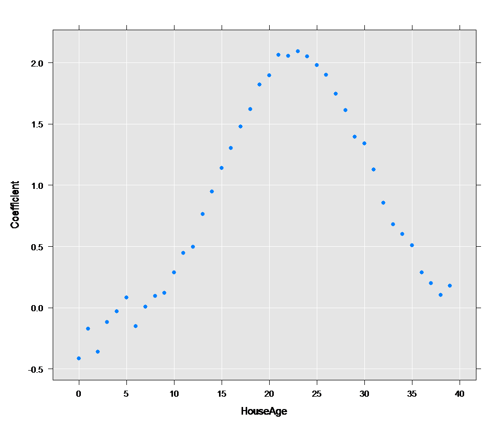
We can extract the coefficients from logitObj for the houseAge variables and plot them:
	cc <- coef(logitObj)
	df <- data.frame(Coefficient=cc[2:41], HouseAge=0:39)
	rxLinePlot(Coefficient~HouseAge,data=df, type="p")
The resulting plot shows that the age of the house is associated with a higher default rate in the middle of the range than for younger and older houses.
Compute the Probability of Default
Using the rxPredict function, we can compute the probability of default for given characteristics using our estimated logistic regression model as input. First create some vectors containing values of interest for each of the independent variables:
	creditScore <- c(300, 700)
	yearsEmploy <- c( 2, 8)
	ccDebt <- c(5000, 10000)
	year <- c(2008, 2009)
	houseAge <- c(5, 20)
Now create a data frame with combinations of those values:
	predictDF <- data.frame(
		creditScore = rep(creditScore, times = 16),
		yearsEmploy = rep(rep(yearsEmploy, each = 2), times = 8),
		ccDebt      = rep(rep(ccDebt, each = 4), times = 4),
		year        = rep(rep(year, each = 8), times = 2),
		houseAge    = rep(houseAge, each = 16))
Using the rxPredict function, we can compute the predicted probability of default for each of the variable combinations. The predicted values will be added to the outData data set, if it already exists:
	predictDF <- rxPredict(modelObject = logitObj, data = predictDF,
	    outData = predictDF)
	predictDF[order(predictDF$default_Pred, decreasing = TRUE),]
The results should be printed to your console, with the highest default rate at the top:
	   creditScore yearsEmploy ccDebt year houseAge default_Pred
	29         300           2  10000 2009       20 9.879328e-01
	21         300           2  10000 2008       20 9.748884e-01
	31         300           8  10000 2009       20 9.377608e-01
	13         300           2  10000 2009        5 9.304742e-01
	23         300           8  10000 2008       20 8.772219e-01
	5          300           2  10000 2008        5 8.638767e-01
	30         700           2  10000 2009       20 8.334778e-01
	15         300           8  10000 2009        5 7.112344e-01
	22         700           2  10000 2008       20 7.035689e-01
	7          300           8  10000 2008        5 5.387369e-01
	32         700           8  10000 2009       20 4.794787e-01
	14         700           2  10000 2009        5 4.500066e-01
	24         700           8  10000 2008       20 3.040133e-01
	6          700           2  10000 2008        5 2.795344e-01
	16         700           8  10000 2009        5 1.308739e-01
	25         300           2   5000 2009       20 6.756520e-02
	8          700           8  10000 2008        5 6.664645e-02
	17         300           2   5000 2008       20 3.321951e-02
	27         300           8   5000 2009       20 1.316013e-02
	9          300           2   5000 2009        5 1.170657e-02
	19         300           8   5000 2008       20 6.284003e-03
	1          300           2   5000 2008        5 5.585628e-03
	26         700           2   5000 2009       20 4.410500e-03
	11         300           8   5000 2009        5 2.175239e-03
	18         700           2   5000 2008       20 2.096317e-03
	3          300           8   5000 2008        5 1.032677e-03
	28         700           8   5000 2009       20 8.146337e-04
	10         700           2   5000 2009        5 7.236564e-04
	20         700           8   5000 2008       20 3.864641e-04
	2          700           2   5000 2008        5 3.432878e-04
	12         700           8   5000 2009        5 1.332594e-04
	4          700           8   5000 2008        5 6.319589e-05
Next steps
- If you missed the first tutorial, see Practice data import and exploration for an overview.
- For more advanced lessons, see Write custom chunking algorithms.