Caution
This article references CentOS, a Linux distribution that is nearing End Of Life (EOL) status. Please consider your use and plan accordingly. For more information, see the CentOS End Of Life guidance.
This article describes the steps for how to run Ansys CFX on a virtual machine (VM) that's deployed on Azure. It also presents the performance results of running Ansys CFX on Azure.
Ansys CFX is computational fluid dynamics (CFD) software for turbomachinery applications. It uses an equilibrium phase change model and relies on material properties to reliably predict cavitation without the need for empirical model parameters. CFX:
Uses transient blade row methods to reduce geometry from a full wheel to a single passage.
Integrates with Geolus Shape Search to rapidly find parts that are identical to a specified part, based on geometry.
CFX is used in the aerospace, defense, steam turbine, energy, automotive, construction, facilities, manufacturing, and materials/chemical processing industries.
Why deploy Ansys CFX on Azure?
- Modern and diverse compute options to align to your workload's needs
- The flexibility of virtualization without the need to buy and maintain physical hardware
- Rapid provisioning
- Multi-node deployment as much as 17 times faster than single-node deployment
Architecture
The following architecture shows a single-node configuration:

Download a Visio file of this architecture.
The following architecture shows a multi-node configuration:

Download a Visio file of this architecture.
Components
- Use Azure Virtual Machines to create a Linux VM. For information about deploying the VM and installing the drivers, see Linux VMs on Azure.
- Use Azure Virtual Network to create a private network infrastructure in the cloud.
- Use network security groups to restrict access to the VM. A public IP address connects the internet to the VM.
- Use Azure CycleCloud to create the cluster in the multi-node configuration.
- Use a physical solid-state drive (SSD) for storage.
Compute sizing and drivers
Performance tests of Ansys CFX on Azure used HBv3-series VMs running Linux. The following table provides the configuration details.
| VM size | vCPU | Memory (GiB) | Memory bandwidth (GBps) | Base CPU frequency (GHz) | All-cores frequency (GHz, peak) | Single-core frequency (GHz, peak) | RDMA performance (Gbps) | Maximum data disks |
|---|---|---|---|---|---|---|---|---|
| Standard_HB120rs_v3 | 120 | 448 | 350 | 2.45 | 3.1 | 3.675 | 200 | 32 |
| Standard_HB120-96rs_v3 | 96 | 448 | 350 | 2.45 | 3.1 | 3.675 | 200 | 32 |
| Standard_HB120-64rs_v3 | 64 | 448 | 350 | 2.45 | 3.1 | 3.675 | 200 | 32 |
| Standard_HB120-32rs_v3 | 32 | 448 | 350 | 2.45 | 3.1 | 3.675 | 200 | 32 |
| Standard_HB120-16rs_v3 | 16 | 448 | 350 | 2.45 | 3.1 | 3.675 | 200 | 32 |
Install Ansys CFX on a VM or HPC cluster
You can download the software from the official Ansys CFX website.
Before you install Ansys CFX, you need to deploy and connect to a VM or HPC cluster.
For information on how to deploy the VM and install the drivers, see the following articles:
For information on how to deploy Azure CycleCloud and the HPC cluster, see the following articles:
CFX performance results
The following tests analyzed the CFD software, Ansys CFX 2021 R2 and Ansys CFX 2022 R2. The following table provides the details of the VM that was used for testing.
| System/software details | HBv3 (Milan) | HBv3 (Milan-X) |
|---|---|---|
| Operating system (OS) version | CentOS-based 8.1 HPC Gen_2 | CentOS-based 8.1 HPC Gen_2 |
| OS architecture | X86-64 | X86-64 |
| Processor | AMD EPYC 7V13 | AMD EPYC 7V73X |
Many factors can influence HPC scalability, including the mesh size, element type, mesh topology, and physical models. To get meaningful and case-specific benchmark results, it's best to use the standard HPC benchmark cases in the Ansys customer portal.
The following models were tested. For more information about the current Ansys models, see Ansys Engineering Simulation Solutions.
The pump model
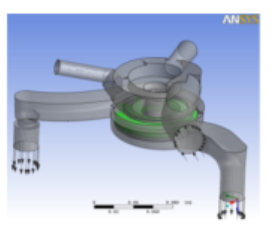
Case details:
Automotive pump with rotating and stationary components
- Turbulent k-e, incompressible, isothermal, multiple frames of reference
- Advection - scheme: specified blend factor 0.75
Global mesh size: 1,305,718 nodes, 5,362,055 elements (Tetrahedra: 4,509,881, Prisms: 850,617, Pyramids: 1557)
Benchmark information:
- Suitable for up to about 16 cores
- Currently set to 10 iterations
- Total solver memory requirement is about 3 GB
The airfoil 10M model
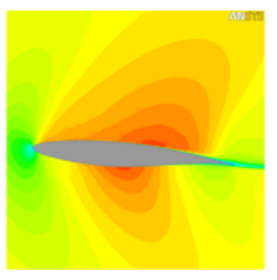
Case details:
Transonic flow around an airfoil. The flow is two-dimensional. The mesh is extruded to provide three-dimensional meshes of various sizes
- Turbulent SST, ideal gas, heat transfer
- Default advection scheme (high resolution)
Global mesh size: 9,933,000 nodes and 9,434,520 elements
Benchmark information:
- Suitable for up to about 50 partitions
- Currently set to 5 iterations
- Partitioning memory requirement is 1.7 GB
- Total solver memory requirement is 13 GB
The airfoil 50M model
Case details:
Transonic flow around an airfoil. The flow is two-dimensional. The mesh is extruded to provide three-dimensional meshes of various sizes.
- Turbulent SST, ideal gas, heat transfer
- Default advection scheme (high resolution)
Global mesh size: 47,773,000 nodes and 47,172,600 elements
Benchmark information:
- Suitable for more than 100 partitions
- Currently set to 5 iterations
- Partitioning memory requirement is about 13 GB
- Total solver memory requirement is about 65 GB
The airfoil 100M model
Case details:
Transonic flow around an Airfoil. The flow is two-dimensional. The mesh is extruded to provide three-dimensional meshes of various sizes.
- Turbulent SST, ideal gas, heat transfer
- Default advection scheme (high resolution)
Global mesh size: 104,533,000 nodes and 103,779,720 elements (all hexahedra)
Benchmark information:
- Suitable for hundreds or thousands of partitions
- Currently set to 5 iterations
- Partitioning memory requirement is about 28 GB
- Total solver memory requirement is about 140 GB
Ansys CFX 2021 R2 performance results on single-node configurations
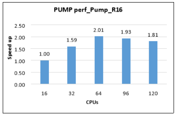
The following table and graph show elapsed wall-clock times and relative speed increases for the pump model.
| Model | Iterations | Cores | CFD solver wall-clock time (seconds) | Relative speed increase |
|---|---|---|---|---|
| perf_Pump_R16 | 10 | 16 | 32.59 | 1.00 |
| perf_Pump_R16 | 10 | 32 | 20.48 | 1.59 |
| perf_Pump_R16 | 10 | 64 | 16.19 | 2.01 |
| perf_Pump_R16 | 10 | 96 | 16.85 | 1.93 |
| perf_Pump_R16 | 10 | 120 | 18.00 | 1.81 |
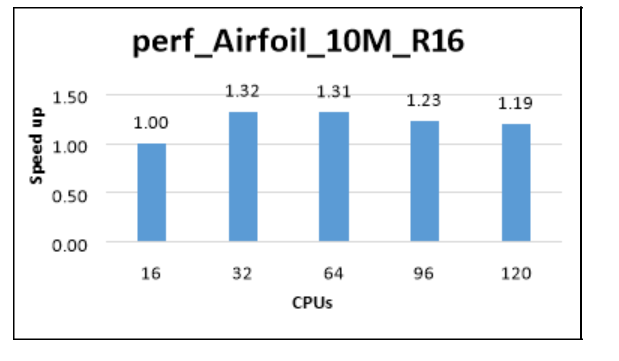
The following table and graph show elapsed wall-clock times and relative speed increases for the airfoil model, with a mesh size of 10 million.
| Model | Iterations | Cores | CFD solver wall-clock time (seconds) | Relative speed increase |
|---|---|---|---|---|
| perf_Airfoil_10M_R16 | 5 | 16 | 149.40 | 1.00 |
| perf_Airfoil_10M_R16 | 5 | 32 | 113.05 | 1.32 |
| perf_Airfoil_10M_R16 | 5 | 64 | 113.87 | 1.31 |
| perf_Airfoil_10M_R16 | 5 | 96 | 121.71 | 1.23 |
| perf_Airfoil_10M_R16 | 5 | 120 | 125.10 | 1.19 |
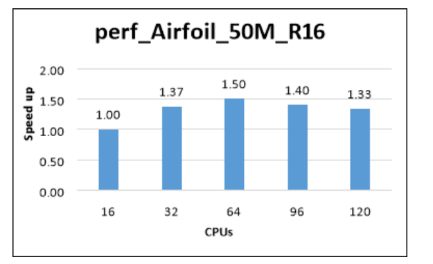
The following table and graph show elapsed wall-clock times and relative speed increases for the airfoil model, with a mesh size of 50 million.
| Model | Iterations | Cores | CFD solver wall-clock time (seconds) | Relative speed increase |
|---|---|---|---|---|
| perf_Airfoil_50M_R16 | 5 | 16 | 861.34 | 1.00 |
| perf_Airfoil_50M_R16 | 5 | 32 | 627.99 | 1.37 |
| perf_Airfoil_50M_R16 | 5 | 64 | 573.76 | 1.50 |
| perf_Airfoil_50M_R16 | 5 | 96 | 616.32 | 1.40 |
| perf_Airfoil_50M_R16 | 5 | 120 | 646.07 | 1.33 |
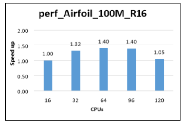
The following table and graph show elapsed wall-clock times and relative speed increases for the airfoil model, with a mesh size of 100 million.
| Model | Iterations | Cores | CFD solver wall-clock time (seconds) | Relative speed increase |
|---|---|---|---|---|
| perf_Airfoil_100M_R16 | 5 | 16 | 2029.20 | 1.00 |
| perf_Airfoil_100M_R16 | 5 | 32 | 1541.70 | 1.32 |
| perf_Airfoil_100M_R16 | 5 | 64 | 1445.70 | 1.40 |
| perf_Airfoil_100M_R16 | 5 | 96 | 1451.70 | 1.40 |
| perf_Airfoil_100M_R16 | 5 | 120 | 1473.70 | 1.05 |
Ansys CFX 2021 R2 and Ansys CFX 2022 R2 performance results on multi-node configurations
The following cluster configuration is based on the single-node results. The single node tests were carried out using AMD Milan processors. The cluster runs used Milan-X AMD processors, which are the latest updated version of AMD EPYC-series processors.
As the single-node results show, scalability improves as the number of cores increases. Because memory bandwidth is fixed on a single node, performance saturates after a certain number of cores is reached. A multi-node configuration surpasses this limitation to fully take advantage of the CFX solver capabilities.
Based on the single-node tests, the 64-CPU configuration is optimal. It's also less expensive than 96-CPU and 120-CPU configurations. The Standard_HB120-64rs_v3 VM with 64 CPUs was used for the multi-node tests.
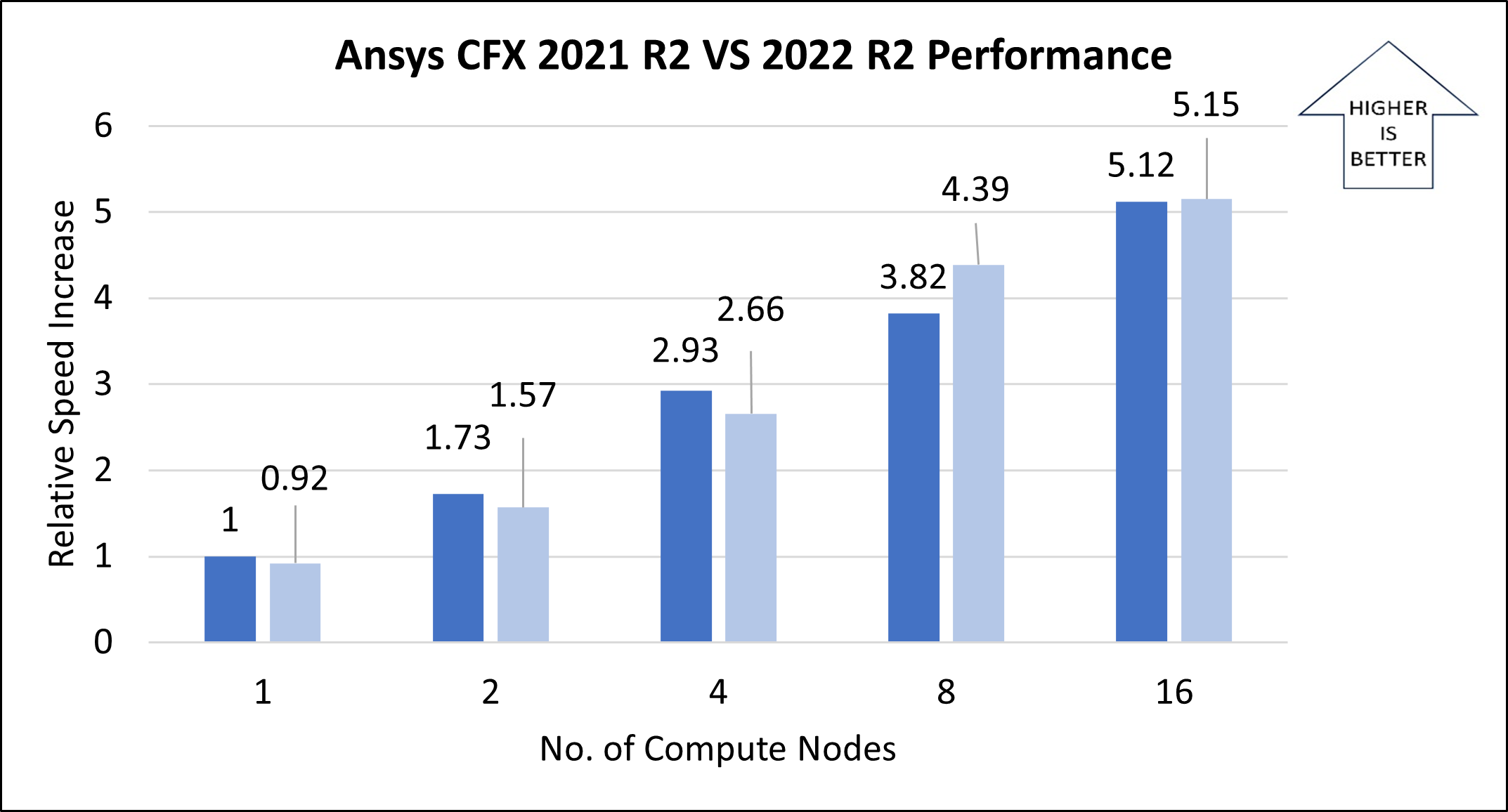
To take advantage of the benefits of the latest processors for CFX simulations, the multi-node tests run on the Milan-X processors. The following results compare the Ansys CFX 2021 R2 and Ansys CFX 2022 R2 versions.
The following table and graph show elapsed wall-clock times and relative speed increases for the pump model, with a stator and rotor assembly.
| Number of nodes | Number of vCPUs | CFD solver wall-clock time, in seconds (2021 R2) | CFD solver wall-clock time, in seconds (2022 R2) | Relative speed increase (2021 R2) | Relative speed increase (2022 R2) | Solver time improvement |
|---|---|---|---|---|---|---|
| 1 | 64 | 11.36 | 12.37 | 1.00 | 0.92 | -8.85% |
| 2 | 128 | 6.56 | 7.256 | 1.73 | 1.57 | -10.61% |
| 4 | 256 | 3.88 | 4.271 | 2.93 | 2.66 | -10.08% |
| 8 | 512 | 2.97 | 2.585 | 3.82 | 4.39 | 12.96% |
| 16 | 1024 | 2.22 | 2.206 | 5.12 | 5.15 | 0.63% |
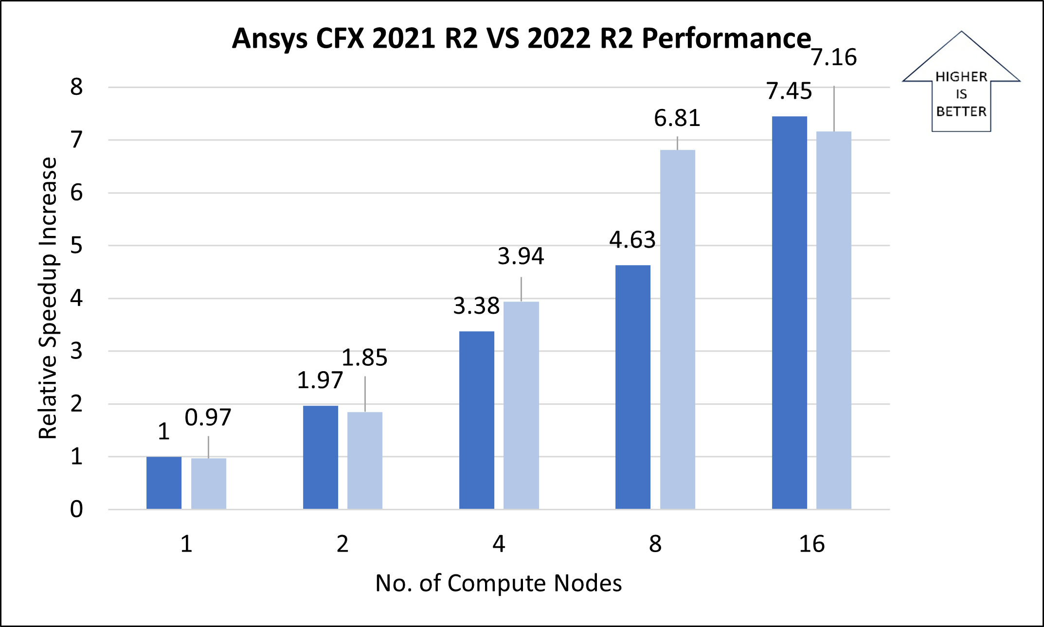
The following table and graph show elapsed wall-clock times and relative speed increases for the airfoil model, with a mesh size of 10 million.
| Number of nodes | Number of vCPUs | CFD solver wall-clock time, in seconds (2021 R2) | CFD solver wall-clock time, in seconds (2022 R2) | Relative speed increase (2021 R2) | Relative speed increase (2022 R2) | Solver time improvement |
|---|---|---|---|---|---|---|
| 1 | 64 | 70.03 | 72.19 | 1.00 | 0.97 | -3.09% |
| 2 | 128 | 35.54 | 37.87 | 1.97 | 1.85 | -6.56% |
| 4 | 256 | 20.71 | 17.80 | 3.38 | 3.94 | 14.07% |
| 8 | 512 | 15.12 | 10.28 | 4.63 | 6.81 | 31.99% |
| 16 | 1024 | 9.4 | 9.79 | 7.45 | 7.16 | -4.11% |
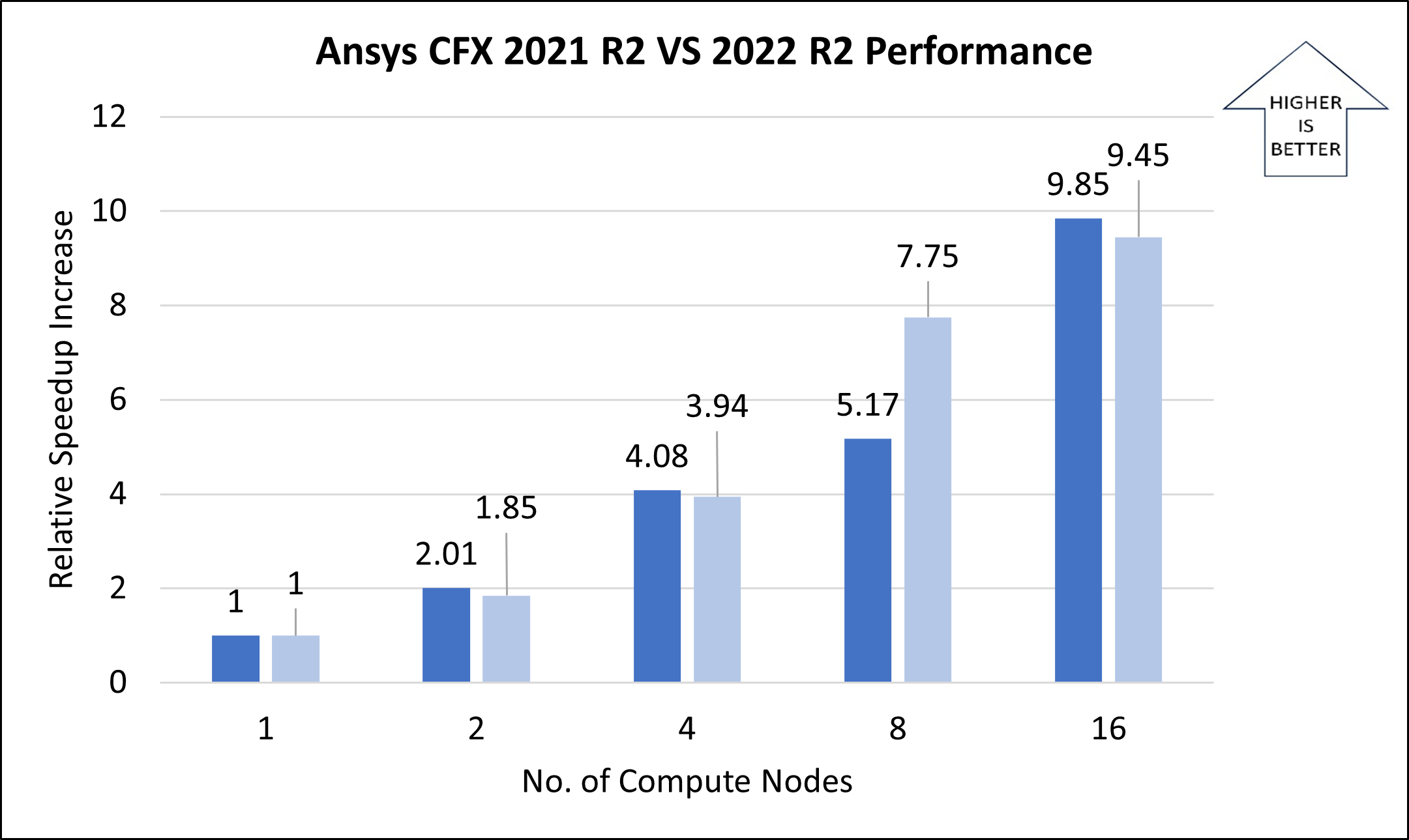
The following table and graph show elapsed wall-clock times and relative speed increases for the airfoil model, with a mesh size of 50 million.
| Number of nodes | Number of vCPUs | CFD solver wall-clock time, in seconds (2021 R2) | CFD solver wall-clock time, in seconds (2022 R2) | Relative speed increase (2021 R2) | Relative speed increase (2022 R2) | Solver time improvement |
|---|---|---|---|---|---|---|
| 1 | 64 | 371.33 | 373.15 | 1.00 | 1.00 | -0.49% |
| 2 | 128 | 184.35 | 201.23 | 2.01 | 1.85 | -9.16% |
| 4 | 256 | 91 | 94.24 | 4.08 | 3.94 | -3.56% |
| 8 | 512 | 71.84 | 47.90 | 5.17 | 7.75 | 33.33% |
| 16 | 1024 | 37.69 | 39.30 | 9.85 | 9.45 | -4.26% |
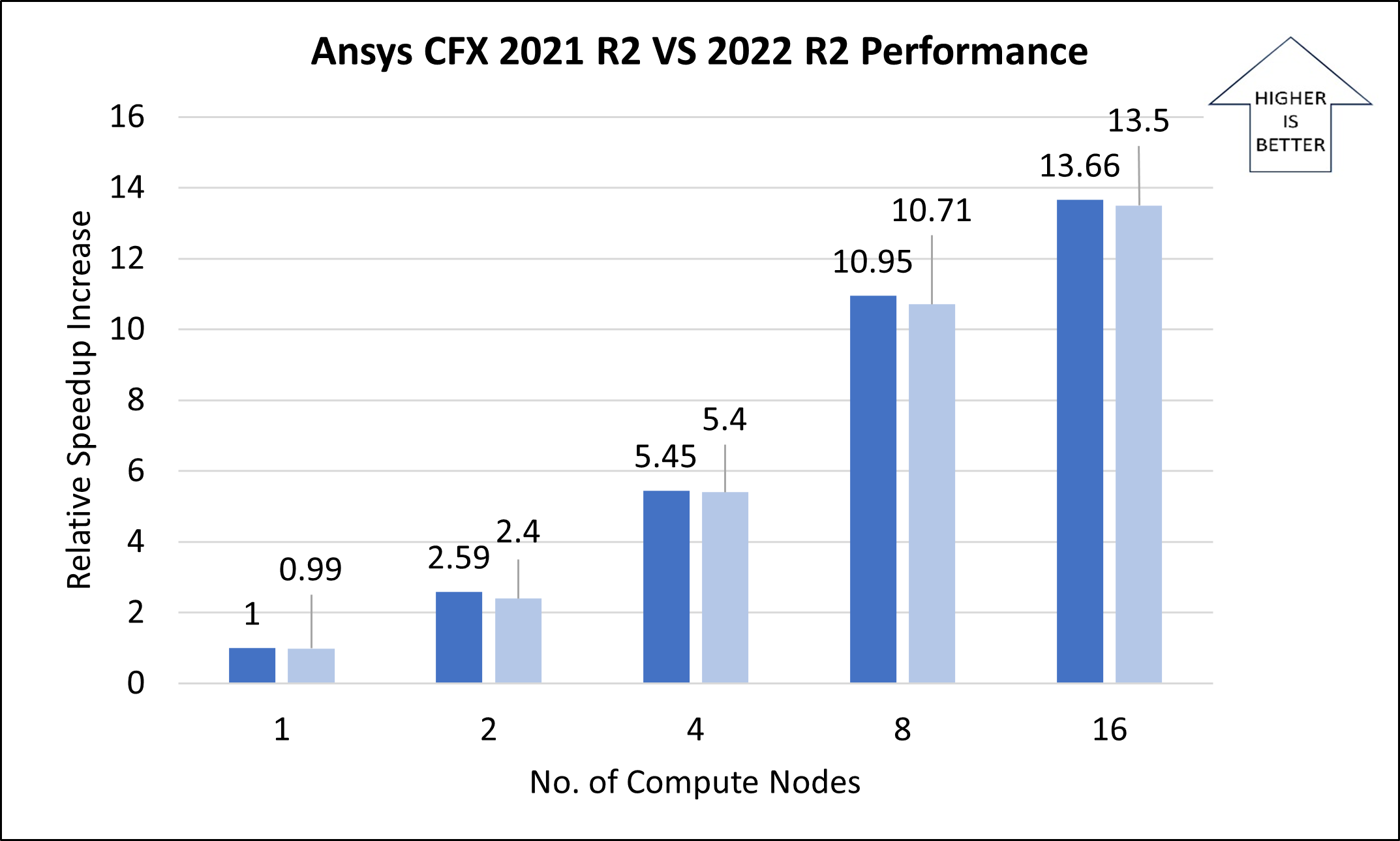
The following table and graph show elapsed wall-clock times and relative speed increases for the airfoil model, with a mesh size of 100 million.
| Number of nodes | Number of vCPUs | CFD solver wall-clock time, in seconds (2021 R2) | CFD solver wall-clock time, in seconds (2022 R2) | Relative speed increase (2021 R2) | Relative speed increase (2022 R2) | Solver time improvement |
|---|---|---|---|---|---|---|
| 1 | 64 | 1139 | 1146.40 | 1.00 | 0.99 | -0.65% |
| 2 | 128 | 439.92 | 473.65 | 2.59 | 2.40 | -7.67% |
| 4 | 256 | 208.92 | 211.07 | 5.45 | 5.40 | -1.03% |
| 8 | 512 | 104 | 106.35 | 10.95 | 10.71 | -2.26% |
| 16 | 1024 | 83.38 | 84.34 | 13.66 | 13.50 | -1.16% |
Azure cost
The following tables provide wall-clock times that you can use to calculate Azure costs. To compute the cost, multiply the wall-clock time by the number of nodes and the Azure VM hourly rate. For the hourly rates for Linux, see Linux VMs pricing. Azure VM hourly rates are subject to change.
Only the simulation runtime is considered for the cost calculations. Installation time, simulation setup time, and software costs aren't included. The time for each configuration in the following tables is the combined wall-clock time for all models.
You can use the Azure pricing calculator to estimate VM costs for your configuration.
Cost for Ansys CFX 2021 R2
| Number of Nodes | Number of vCPUs | Time, in hours |
|---|---|---|
| 1 | 64 | 0.44 |
| 2 | 128 | 0.18 |
| 4 | 256 | 0.09 |
| 8 | 512 | 0.053 |
| 16 | 1024 | 0.036 |
Cost for Ansys CFX 2022R2
| Number of nodes | Number of vCPUs | Time, in hours |
|---|---|---|
| 1 | 64 | 0.45 |
| 2 | 128 | 0.20 |
| 4 | 256 | 0.09 |
| 8 | 512 | 0.05 |
| 16 | 1,024 | 0.04 |
Summary
Ansys CFX 2021 R2 and Ansys CFX 2022 R2 were both successfully deployed and tested on HBv3 120 AMD EPYC™ 7V73X-series (Milan-X) VMs.
- For a single-node configuration, there's a relative speed increase up to 64 cores. There's no relative speed increase for more than 64 cores.
- For a multi-node configuration, with sufficiently large models, Ansys CFX scales up linearly with each increase in the number of nodes.
- There's a relative speed increase of about 13.5 times with a multi-node configuration (16 nodes) for a considerably large model (100 million cells). These results indicate that Ansys CFX performs well on Azure HBv3 VMs.
- The preceding test results show the performance of Ansys CFX 2021 R2 compared to Ansys CFX 2022 R2.
Contributors
This article is maintained by Microsoft. It was originally written by the following contributors.
Principal authors:
- Hari Bagudu | Senior Manager
- Gauhar Junnarkar | Principal Program Manager
- Vinod Pamulapati | HPC Performance Engineer
Other contributors:
- Guy Bursell | Director Business Strategy
- Sachin Rastogi | Manager
To see non-public LinkedIn profiles, sign in to LinkedIn.
Next steps
- GPU-optimized VM sizes
- VMs on Azure
- Virtual networks and VMs on Azure
- Learning path: Run high-performance computing (HPC) applications on Azure