Excel
Microsoft Excel is a tool for creating spreadsheets, calculations, graphs, and charts. People of all abilities can understand your data more easily if you create Excel workbooks and charts with accessibility in mind.
Column headers
Column headers make it easy to navigate through a table with a large amount of data. Most screen readers will read out column headers when in a cell within the table. For example, if a screen reader is in the third row of a data table, it can refer back to the column header so the person using it knows the context of the data they're hearing.
To create a table with column headers:
- Select Insert > Table.
- Highlight the cells that correspond to that table or the cells where your table will go.
- Check the My table has headers box in the Create Table dialog.
- Ensure the specified column headers have unique names. By default, Excel will name these Column 1, Column 2, and so on.

Sheet names
People who use screen readers can navigate among tabs using the keyboard. Tab names make it easy to determine where they are in the workbook.
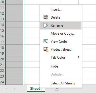
To create, edit, and style tab names:
- Right-click on the sheet tab and select Rename, or move to the desired sheet and select Home > Format > Rename sheet. You can also change tab color in the format menu.
- Enter a unique name for the sheet.
Charts and graphs
Accessible design can still be stylish and visually appealing. You can use colors and styles to create your Excel charts and graphs, but also provide an alternative. Text and data tables are good alternatives or supplements to charts and graphs, because they're linear and easily navigable with a screen reader.
They're also helpful for people who might not understand the topic or who have cognitive disabilities. For example, some people might struggle to understand text and data in a table, and a clearly marked chart can help them to better grasp the information being communicated.
To add chart labels:
- Chart title: After you create the chart, adjust the title to ensure it's descriptive and meaningful to the chart content.
- Axis titles: Select the chart, then select the Chart Design tab > Add Chart Element > Axis Titles. Ensure the Axis Title clearly describes the axis.
- Data labels: Select the chart, then select the Chart Design tab > Add Chart Element > Data Labels > Outside End.

To create an accessible chart design:
- Adjust colors to ensure good contrast between labels and data points.
- Use patterns rather than solid colors if possible.
- Add alternative text to the chart. Select the chart, then right-click or press the applications key. Select View Alt Text. Enter a meaningful description of the chart.
- Use a sans serif font and a font size of 12 points or greater.
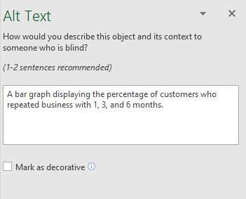
Table name
Always give a table a unique name so that a person using a screen reader can easily differentiate among data tables. Be sure to not use spaces or special characters in the table name, only letters and numbers. If someone is using a screen reader, the unique table names will help them differentiate among tables.
To edit a table name:
- Select a cell within the table.
- Select the Table Design tab.
- In the Properties section, enter a unique table name that doesn't include spaces or special characters.
