Exercise - Clean and prepare data - Training

10 minutes

Before you can prepare a dataset, you need to understand its content and structure. In the previous lab, you imported a dataset containing on-time arrival information for a major U.S. airline. That data included 26 columns and thousands of rows, with each row representing one flight and containing information such as the flight's origin, destination, and scheduled departure time. You also loaded the data into a Jupyter notebook and used a simple Python script to create a Pandas DataFrame from it.

A DataFrame is a two-dimensional labeled data structure. The columns in a DataFrame can be of different types, just like columns in a spreadsheet or database table. It is the most commonly used object in Pandas. In this exercise, you will examine the DataFrame — and the data inside it — more closely.

Switch back to the Azure notebook that you created in the previous section. If you closed the notebook, you can sign back into the Microsoft Azure Notebooks portal, open your notebook and use the Cell -> Run All to rerun the all of the cells in the notebook after opening it.

The FlightData notebook
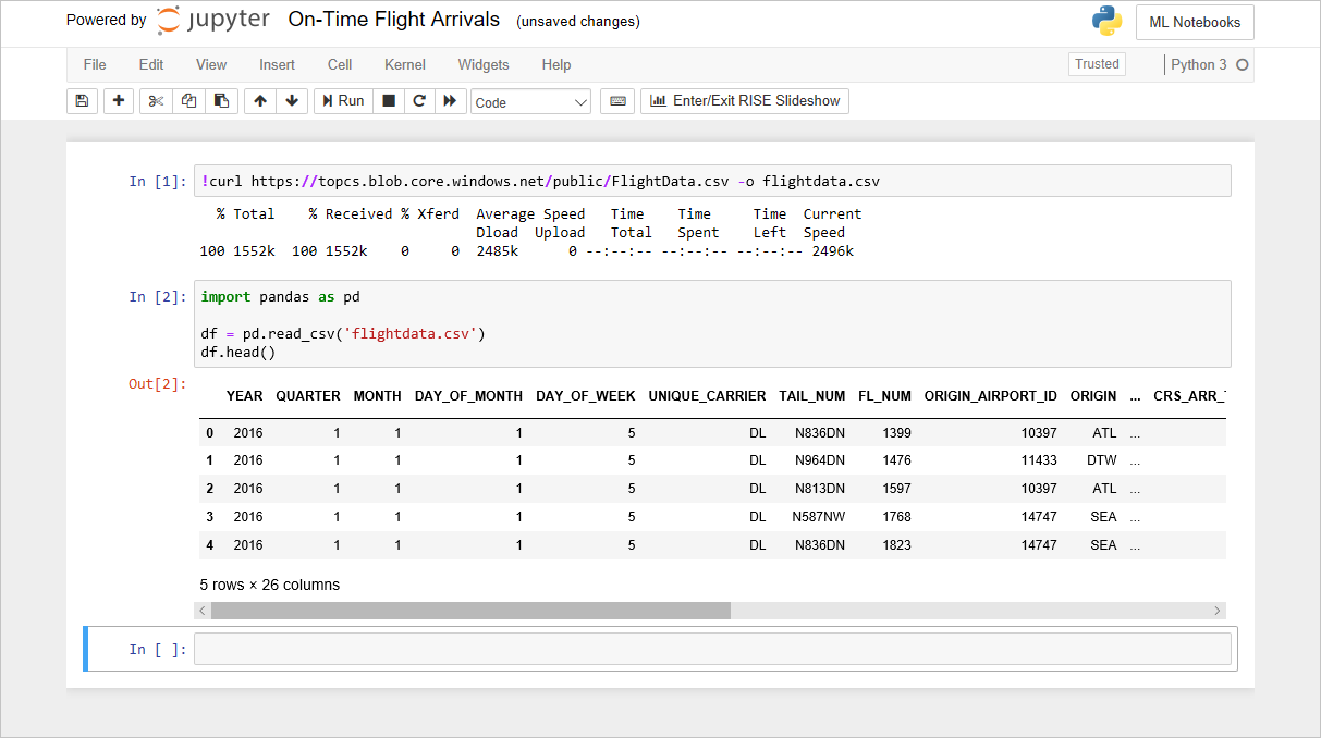
The code that you added to the notebook in the previous lab creates a DataFrame from flightdata.csv and calls DataFrame.head on it to display the first five rows. One of the first things you typically want to know about a dataset is how many rows it contains. To get a count, type the following statement into an empty cell at the end of the notebook and run it:
```
df.shape
```
Confirm that the DataFrame contains 11,231 rows and 26 columns:

Getting a row and column count

Now take a moment to examine the 26 columns in the dataset. They contain important information such as the date that the flight took place (YEAR, MONTH, and DAY_OF_MONTH), the origin and destination (ORIGIN and DEST), the scheduled departure and arrival times (CRS_DEP_TIME and CRS_ARR_TIME), the difference between the scheduled arrival time and the actual arrival time in minutes (ARR_DELAY), and whether the flight was late by 15 minutes or more (ARR_DEL15).

Here is a complete list of the columns in the dataset. Times are expressed in 24-hour military time. For example, 1130 equals 11:30 a.m. and 1500 equals 3:00 p.m.

Column	Description
YEAR	Year that the flight took place
QUARTER	Quarter that the flight took place (1-4)
MONTH	Month that the flight took place (1-12)
DAY_OF_MONTH	Day of the month that the flight took place (1-31)
DAY_OF_WEEK	Day of the week that the flight took place (1=Monday, 2=Tuesday, etc.)
UNIQUE_CARRIER	Airline carrier code (e.g., DL)
TAIL_NUM	Aircraft tail number
FL_NUM	Flight number
ORIGIN_AIRPORT_ID	ID of the airport of origin
ORIGIN	Origin airport code (ATL, DFW, SEA, etc.)
DEST_AIRPORT_ID	ID of the destination airport
DEST	Destination airport code (ATL, DFW, SEA, etc.)
CRS_DEP_TIME	Scheduled departure time
DEP_TIME	Actual departure time
DEP_DELAY	Number of minutes departure was delayed
DEP_DEL15	0=Departure delayed less than 15 minutes, 1=Departure delayed 15 minutes or more
CRS_ARR_TIME	Scheduled arrival time
ARR_TIME	Actual arrival time
ARR_DELAY	Number of minutes flight arrived late
ARR_DEL15	0=Arrived less than 15 minutes late, 1=Arrived 15 minutes or more late
CANCELLED	0=Flight was not cancelled, 1=Flight was cancelled
DIVERTED	0=Flight was not diverted, 1=Flight was diverted
CRS_ELAPSED_TIME	Scheduled flight time in minutes
ACTUAL_ELAPSED_TIME	Actual flight time in minutes
DISTANCE	Distance traveled in miles

The dataset includes a roughly even distribution of dates throughout the year, which is important because a flight out of Minneapolis is less likely to be delayed due to winter storms in July than it is in January. But this dataset is far from being "clean" and ready to use. Let's write some Pandas code to clean it up.

One of the most important aspects of preparing a dataset for use in machine learning is selecting the "feature" columns that are relevant to the outcome you are trying to predict while filtering out columns that do not affect the outcome, could bias it in a negative way, or might produce multicollinearity. Another important task is to eliminate missing values, either by deleting the rows or columns containing them or replacing them with meaningful values. In this exercise, you will eliminate extraneous columns and replace missing values in the remaining columns.

One of the first things data scientists typically look for in a dataset is missing values. There's an easy way to check for missing values in Pandas. To demonstrate, execute the following code in a cell at the end of the notebook:
```
df.isnull().values.any()
```
Confirm that the output is "True," which indicates that there is at least one missing value somewhere in the dataset.

Checking for missing values
The next step is to find out where the missing values are. To do so, execute the following code:
```
df.isnull().sum()
```
Confirm that you see the following output listing a count of missing values in each column:

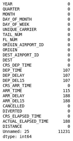
Number of missing values in each column
Curiously, the 26th column ("Unnamed: 25") contains 11,231 missing values, which equals the number of rows in the dataset. This column was mistakenly created because the CSV file that you imported contains a comma at the end of each line. To eliminate that column, add the following code to the notebook and execute it:
```
df = df.drop('Unnamed: 25', axis=1)
df.isnull().sum()
```
Inspect the output and confirm that column 26 has disappeared from the DataFrame:

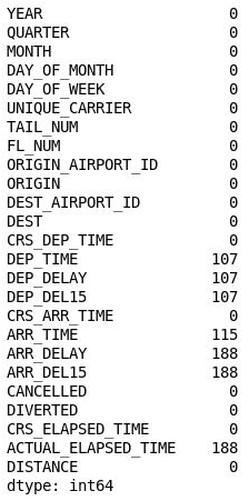
The DataFrame with column 26 removed
The DataFrame still contains a lot of missing values, but some of them aren't useful because the columns containing them are not relevant to the model that you are building. The goal of that model is to predict whether a flight you are considering booking is likely to arrive on time. If you know that the flight is likely to be late, you might choose to book another flight.

The next step, therefore, is to filter the dataset to eliminate columns that aren't relevant to a predictive model. For example, the aircraft's tail number probably has little bearing on whether a flight will arrive on time, and at the time you book a ticket, you have no way of knowing whether a flight will be cancelled, diverted, or delayed. By contrast, the scheduled departure time could have a lot to do with on-time arrivals. Because of the hub-and-spoke system used by most airlines, morning flights tend to be on time more often than afternoon or evening flights. And at some major airports, traffic stacks up during the day, increasing the likelihood that later flights will be delayed.

Pandas provides an easy way to filter out columns you don't want. Execute the following code in a new cell at the end of the notebook:
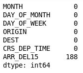
```
df = df[["MONTH", "DAY_OF_MONTH", "DAY_OF_WEEK", "ORIGIN", "DEST", "CRS_DEP_TIME", "ARR_DEL15"]]
df.isnull().sum()
```
The output shows that the DataFrame now includes only the columns that are relevant to the model, and that the number of missing values is greatly reduced:

The filtered DataFrame
The only column that now contains missing values is the ARR_DEL15 column, which uses 0s to identify flights that arrived on time and 1s for flights that didn't. Use the following code to show the first five rows with missing values:
```
df[df.isnull().values.any(axis=1)].head()
```
Pandas represents missing values with NaN, which stands for Not a Number. The output shows that these rows are indeed missing values in the ARR_DEL15 column: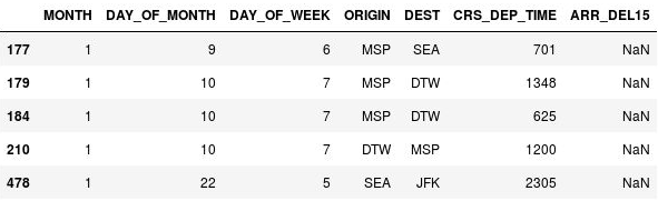

Rows with missing values
The reason these rows are missing ARR_DEL15 values is that they all correspond to flights that were canceled or diverted. You could call dropna on the DataFrame to remove these rows. But since a flight that is canceled or diverted to another airport could be considered "late," let's use the fillna method to replace the missing values with 1s.

Use the following code to replace missing values in the ARR_DEL15 column with 1s and display rows 177 through 184:
```
df = df.fillna({'ARR_DEL15': 1})
df.iloc[177:185]
```
Confirm that the NaNs in rows 177, 179, and 184 were replaced with 1s indicating that the flights arrived late: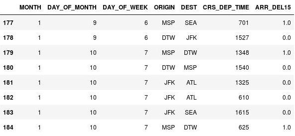

NaNs replaced with 1s

The dataset is now "clean" in the sense that missing values have been replaced and the list of columns has been narrowed to those most relevant to the model. But you're not finished yet. There is more to do to prepare the dataset for use in machine learning.

The CRS_DEP_TIME column of the dataset you are using represents scheduled departure times. The granularity of the numbers in this column — it contains more than 500 unique values — could have a negative impact on accuracy in a machine-learning model. This can be resolved using a technique called binning or quantization. What if you divided each number in this column by 100 and rounded down to the nearest integer? 1030 would become 10, 1925 would become 19, and so on, and you would be left with a maximum of 24 discrete values in this column. Intuitively, it makes sense, because it probably doesn't matter much whether a flight leaves at 10:30 a.m. or 10:40 a.m. It matters a great deal whether it leaves at 10:30 a.m. or 5:30 p.m.

In addition, the dataset's ORIGIN and DEST columns contain airport codes that represent categorical machine-learning values. These columns need to be converted into discrete columns containing indicator variables, sometimes known as "dummy" variables. In other words, the ORIGIN column, which contains five airport codes, needs to be converted into five columns, one per airport, with each column containing 1s and 0s indicating whether a flight originated at the airport that the column represents. The DEST column needs to be handled in a similar manner.

In this exercise, you will "bin" the departure times in the CRS_DEP_TIME column and use Pandas' get_dummies method to create indicator columns from the ORIGIN and DEST columns.

Use the following command to display the first five rows of the DataFrame:
```
df.head()
```
Observe that the CRS_DEP_TIME column contains values from 0 to 2359 representing military times.

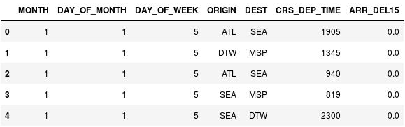
The DataFrame with unbinned departure times
Use the following statements to bin the departure times:
```
import math

for index, row in df.iterrows():
    df.loc[index, 'CRS_DEP_TIME'] = math.floor(row['CRS_DEP_TIME'] / 100)
df.head()
```
Confirm that the numbers in the CRS_DEP_TIME column now fall in the range 0 to 23:

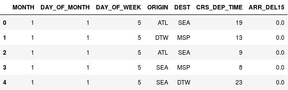
The DataFrame with binned departure times
Now use the following statements to generate indicator columns from the ORIGIN and DEST columns, while dropping the ORIGIN and DEST columns themselves:
```
df = pd.get_dummies(df, columns=['ORIGIN', 'DEST'])
df.head()
```
Examine the resulting DataFrame and observe that the ORIGIN and DEST columns were replaced with columns corresponding to the airport codes present in the original columns. The new columns have 1s and 0s indicating whether a given flight originated at or was destined for the corresponding airport.

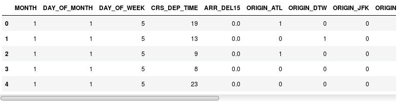
The DataFrame with indicator columns
Use the File -> Save and Checkpoint command to save the notebook.

The dataset looks very different than it did at the start, but it is now optimized for use in machine learning.

Continue

Exercise - Clean and prepare data

Feedback