Removing VSTO-Based Customizations from a PowerPivot Workbook
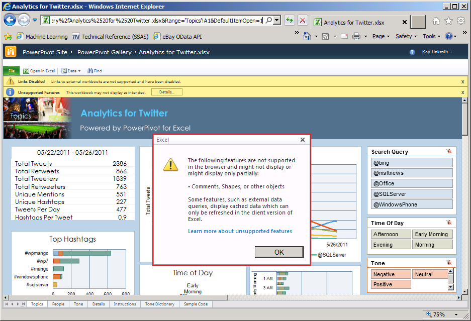
This article is a follow-up on a previous blog post titled “How to Build a VSTO-Based PowerPivot Workbook,” which discussed some of the advantages and disadvantages of building PowerPivot workbooks by using VSTO. A key VSTO advantage is that you can bring data from virtually any source into PowerPivot even if there is no suitable data provider, but a significant disadvantage is that Excel Services in SharePoint doesn’t run the VSTO code. Among other things, this means that you cannot keep VSTO-based workbooks automatically updated by using the Scheduled Data Refresh feature of PowerPivot for SharePoint. Moreover, Excel Services displays warnings about unsupported and disabled features when viewing the workbook in the browser, such as for buttons, text boxes, and other such objects, as illustrated in the following screenshot, which shows the VSTO-based Analytics for Twitter workbook in Internet Explorer. Removing the VSTO customizations could help to improve the user experience, but how do you bring custom data into a PowerPivot workbook without VSTO if there is no direct data provider?
Converting a VSTO-based PowerPivot workbook into a non-VSTO version—such as to provide seamless browser access and to take advantage of Scheduled Data Refresh in SharePoint—requires the following high-level steps:
- Devise a new import method to get data into PowerPivot without using VSTO.
- Update the workbook’s PowerPivot model to use the new data import method.
- Update the Excel workbook features and remove the VSTO code from the workbook.
Let’s take a closer look at these steps by converting the Analytics for Twitter solution. It is an excellent example that highlights many important PowerPivot elements and their dependencies.
Step 1: Importing data without using VSTO
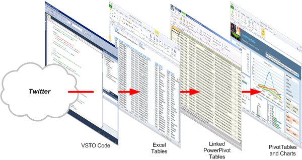
VSTO-based PowerPivot workbooks rely on VSTO customizations primarily to pull data into Excel tables. Linked to PowerPivot tables, these Excel tables then simply act as PowerPivot data sources. Here’s the relevant figure from the previous blog post, which shows the data flow for the Twitter Analytics workbook.
Given the objective to eliminate the VSTO code on the client, we need to replace the Excel tables with a server-based repository that PowerPivot directly supports as a data source, such as a SQL Server database, text files on a file server, or SharePoint lists. The new data import solution can then periodically pull data from Twitter into the chosen server-based repository and PowerPivot can import the data from this repository without the need for VSTO.
The following figure illustrates the import method I chose for this article, which is based on a SharePoint Timer job and a collection of SharePoint lists. I chose this approach because it is relatively straightforward to create a Timer job to retrieve data at a configurable interval from the source and put it into one or multiple lists. PowerPivot can then import these lists through a data feed. For details about how this works, I recommend reading Uday Unni’s excellent white paper “Using SharePoint List Data in PowerPivot” available on MSDN at https://go.microsoft.com/fwlink/?LinkId=221005.
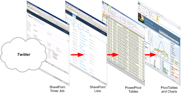
The new data flow is very similar to the original VSTO-based approach. My Timer job just takes on the role of the original VSTO code and the SharePoint lists simply replace the original Excel tables, as already explained. That’s all there is to it. In fact, I asked Analytics for Twitter author Aaron Meyers for permissions to reuse his original code. The source code is included in the Twitter workbook on the Sample Code worksheet. Reusing this code gave me a great head start. Thanks again for sharing, Aaron!
Without going into too much detail about SharePoint programming, here’s how I created my Timer job:
- Installed a developer workstation running SharePoint 2010, PowerPivot for SharePoint, and Visual Studio 2010 with Tools for SharePoint Development.
- Started Visual Studio with elevated permissions and created an initial SharePoint Timer job project according to the steps outlined in the technical article “How to: Create a Web Application-Scoped Timer Job” on MSDN at https://msdn.microsoft.com/en-us/library/ff798313.aspx.
- Copied Aaron’s source code files into the project and modified TwitterSearch.cs so that it would compile. This mainly required commenting out Excel-specific code that is no longer needed and changing some private into protected members to make them accessible in a derived class.
- Derived a TwitterSearchListImport class from the TwitterSearch class to implement the SharePoint-specific logic and updated the Timer job definition to perform data imports into my SharePoint lists.
Note: You can find the resulting Visual Studio project called TwitterImportTimerJob in the attachments to this article. The solution is not optimized for performance. It is for demonstration purposes only and not to be used in a production environment.
You can deploy the solution on a SharePoint developer workstation directly in Visual Studio 2010. By default, the Twitter Import Timer job is configured to run daily between midnight and one o’clock in the morning, but it’s also possible to run this job on demand at any time. In SharePoint Central Administration, click on Monitoring, click on Review Job Definitions, then click on Twitter Import Timer Job, and then in the Timer Job configuration click on Run Now. The following figure shows the results for a run in my test environment.
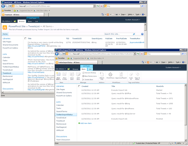
When running the Twitter Import Timer job for the first time, it creates all necessary SharePoint lists automatically, as summarized in the following table.
SharePoint List |
Replaces |
Comments |
TwitterImportStatus |
Message boxes that the Excel client displays during the interactive import process |
The Twitter Import Timer job runs unattended and can’t display message boxes, so it reports processing status and error messages in the TwitterImportStatus list instead. |
SearchTerms |
Text box for comma-separated search queries on the Topics, People, Tone, and Details worksheets |
The Twitter Import Timer job automatically creates the default search terms in the SearchTerms list. You can add and remove search terms to customize the Twitter import process. Each search term item also has an Include property that you can set to No to exclude the term from the searches without deleting it. |
ToneDictList |
tblToneDict table on the Tone Dictionary worksheet |
The Twitter Import Timer job initializes the ToneDictList with the same entries found in the tblToneDict table. |
TweetsList |
tblTweets table on the hidden TweetData worksheet |
The TweetsList columns are almost identical to the tblTweets table, except that TweetGUID replaces the GUID column and TweetAuthor replaces the Author column. |
MentionsList |
tblMentions table on the hidden TweetData worksheet |
The MentionsList has the same columns as the tblMentions table in the workbook. |
HashtagsList |
tblHashtags table on the hidden TweetData worksheet |
The HashtagsList has the same columns as the tblHashtags table in the workbook. |
UtilityList |
tblUtility table on the hidden TweetData worksheet |
The UtilityList has the same columns as the tblUtility table in the workbook. |
Step 2: Updating the PowerPivot model
Ultimately, this step is about replacing the original tables in the workbook’s underlying PowerPivot model with new versions that connect to the corresponding SharePoint lists as their data sources. However, if you simply remove the existing tables, you lose their associated column definitions and measures. It is therefore a good idea to first document the existing PowerPivot model (see TwitterAnalyticsModel.xslx in the attachment to this article for a completed example). It is also a good idea to keep a copy of the original PowerPivot workbook so that you can refer back to the original model if necessary.
There are several important PowerPivot elements in the Twitter Analytics workbook, which the model documentation should cover:
- Table relationships Click on the Design tab in the PowerPivot window and then click Manage Relationships. Document the relationships as displayed and then click Close.
- Table columns In the PowerPivot window, in Data View, go through each table and document for each column the name, data type, and format, as well as the DAX formula for every calculated column.
- Explicit Measures Assuming that you are working with the SQL Server 2012 version of PowerPivot for Excel, it’s straightforward to document the measures because they are displayed in the Calculation Area of each table. Otherwise, you must work with the PowerPivot Field List in the Excel client. Either way, document the measures as you go through each table.
- Implicit measures In addition to explicit measures, you must also document any implicit measures that the PivotTables in the Excel workbook created in response to dragging fields to the Values list in the PowerPivot Field List. You can display these measures in the Calculation Area in Advanced Mode. Just select the option Show Implicit Measures on the Advanced tab. Again, go through each PowerPivot table to document the implicit measures. Their DAX formulas are ready only and cannot be copied, so make sure you document them exactly as shown because you need these formulas later to define explicit measures in the updated PowerPivot model.
Having thoroughly documented the PowerPivot model, you are ready for the ultimate task, which is to replace the existing PowerPivot tables with new versions. First, remove the existing tables, but leave the tblDimDate and tbleDimHour tables in place because these are linked to static Excel tables that don’t have VSTO dependencies. The VSTO code doesn’t update tblDimDate or tblDimHour. Next, follow this procedure to create new tables that use SharePoint lists as their data sources:
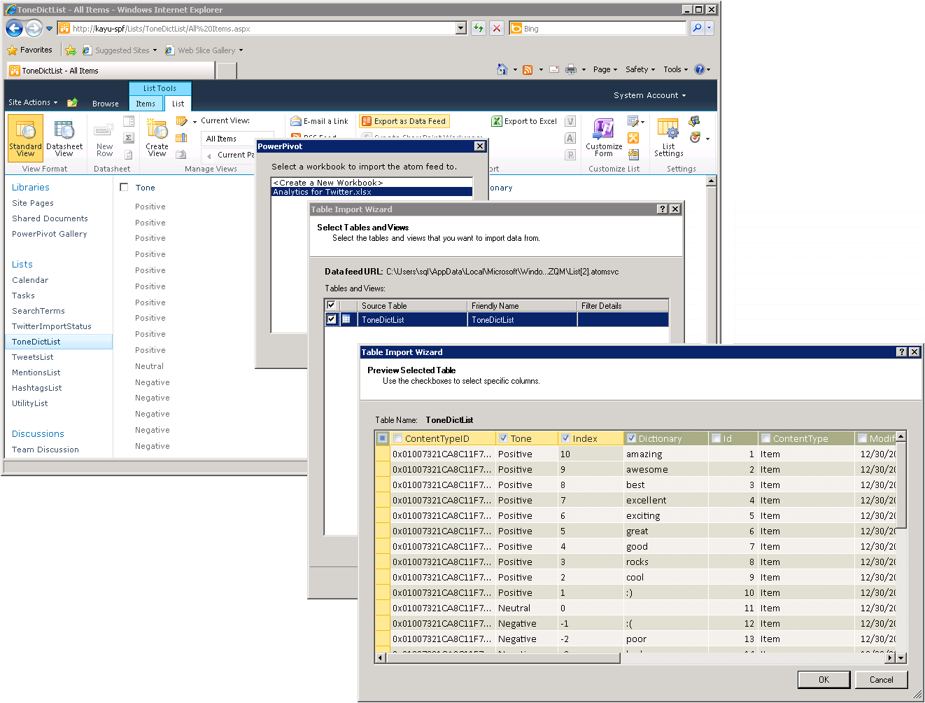
- Make sure you have the Analytics for Twitter.xlsx open in Excel, then go to your SharePoint site and open the ToneDictList in the browser.
- On the SharePoint ribbon, click on List, and then click on Export as Data Feed.
- In the File Download dialog box, click Open.
- In the PowerPivot dialog box, verify that Analytics for Twitter.xlsx is selected, and then click OK.
- In the Table Import Wizard, under Friendly Connection Name, type the name of the SharePoint list, such as ToneDictList, and click Next.
- On the Select Tables and Views page of the Table Import Wizard, verify that the list is selected, and then click Preview & Filter.
- Deselect all SharePoint system columns. In other words, import only the following columns:
Table |
Columns |
ToneDictList |
Tone Index Dictionary |
TweetsList |
Title TID TweetGUID SearchQuery PubDate PrevPubDate TweetAuthor ToneScore |
MentionsList |
Username UID |
HashtagsList |
Hashtag HID |
UtilityList |
TID HID UID |
- Click OK and then click Finish.
- Verify that the import completes successfully and then click Close.
- Right-click the name of the new table and click Rename. Specify the name as follows:
Table |
New Name |
ToneDictList |
tblToneDict |
TweetsList |
tblTweets |
MentionsList |
tblMentions |
HashtagsList |
tblHashtags |
UtilityList |
tblUtility |
- Repeat this procedure for the remaining lists TweetsList, MentionsList, HashtagsList, and UtilityList.
- Save the changes to the Twitter analytics workbook.
The final step is to reapply the original columns and measures to the new tables as previously documented to ensure that all columns are identical to their original versions, that the calculations work, and that all the required table relationships and measures exist. The following procedure yields the desired result:
- Start with the tblToneDict table and convert the data type of the Index column to Whole Number.
- Next, continue with the tblTweets table as follows:
- Convert the data types as in the original tblTweets table according to your model documentation.
- Rename the column TweetGUID into GUID, TweetAuthor into Author, and ToneScore into Tone Score, and SearchQuery into Search Query.
- Add the calculated columns. The last two calculated columns Tone and TimeOfDay will display error messages because the table relationships do not yet exist. This is OK.
- Now, reestablish the table relationships according to your model documentation and verify that the Tone and TimeOfDay columns in the tblTweets table no longer show an error. Assuming that you are working with the latest version of SQL Server 2012 PowerPivot for Excel 2010, you can use the new Diagram View for this purpose. Otherwise, click on Manage Relationship on the Design ribbon to create the relationships.
- Next, edit the tblMentions table to adjust the data type of the UID column and add the calculated MentionCount column according to your model documentation, then update the data types in the tblHashtags tables, and then finish this part of the work by converting the columns in the tblUtility table to the Whole Number data type and adding the calculated columns as outlined in your model documentation.
- Finally, add all explicit measures as well as all implicit measures marked as “In Use” in your model documentation to their associated PowerPivot tables. Recreating the implicit measures as explicit measures in the updated model ensures that the PivotTables and cell formulas in the Excel workbook don’t break. The updated model is not exactly identical to the original version anymore, but this is OK because implicit and explicit measures are the same as far as queries are concerned. It’s just substantially easier to redefine these measures explicitly than to reconfigure the PivotTables in the Excel workbook to recreate them implicitly.
- Don’t forget to save your changes.
Step 3: Updating the Workbook and Removing the VSTO code
At this point, you have completed the PowerPivot work so you can close the PowerPivot window. What’s left is to update the workbook data in Excel according to the following procedure:
- Display the worksheets Topics_Pivot, People_Pivot, and Tone_Pivot by right-clicking a worksheet tab at the bottom of the Excel window and selecting Unhide. In the Unhide dialog box, select the worksheets one at a time and then click OK.
- Switch to the Topics_Pivot worksheet and select a PivotTable to display the PowerPivot Field List. If the field list doesn’t appear automatically, click Field List on the PowerPivot ribbon.
- Notice the warning in the PowerPivot Field List that the PowerPivot data was modified. Click Refresh. If Excel displays a dialog box asking you to replace the contents of destination cells, click OK.
- Check the PivotTables on the People_Pivot, Tone_Pivot, and Details worksheets and repeat steps 2 and 3 if necessary.
- Hide the Topics_Pivot, People_Pivot, and Tone_Pivot worksheets again by right-clicking the corresponding worksheet tab at the bottom and selecting Hide.
- Display the Data ribbon in Excel and click on Refresh All to fully refresh the workbook one more time, then save your changes.
The final task is to remove the VSTO code and clean up the workbook so that it renders without warnings in Excel Services (a completed workbook is attached to this article). Here are the steps:
- In order to remove VSTO, follow the article “How to: Remove Managed Code Extensions from Documents” on MSDN at https://msdn.microsoft.com/en-us/library/bb772099.aspx.
- Open the workbook in Excel, then click on File and Options, and then on the Customize Ribbon tab, select the Developer checkbox to display the Developer ribbon. Click OK.
- Switch to the Developer tab, enable Design Mode, and then remove the buttons and UI elements in the header areas of the Topics, People, Tone, and Details worksheets to specify search terms. Disable Design Mode again and save your changes.
- On each worksheet, remove the remaining unsupported graphical elements, such as the divider line between header and content areas, and the artificial shadow elements around the upper left summary region.
- On the Topics worksheet, also delete the Tweet Type and Tone textboxes placed on top of the bottom PivotCharts. Select the left of these two charts, display the Layout ribbon, click on Chart Title, select Centered Overlay Title, and then type Tweet Type, and place the heading in the original position. Repeat this step for the Tone chart title.
- Display the Formulas tab, and click Name Manager. Remove all named elements with invalid references or references to external resources. Click Close.
- Delete any obsolete worksheets as they might contain elements that Excel Services cannot render. For example, right-click the Sample Code worksheet tab and click Delete. In the Microsoft Excel dialog asking you to confirm that you want to delete this worksheet, click Delete. However, leave the following worksheets in the workbook: Topics, Topic_Pivot, People, People_Pivot, Tone, Tone_Pivot, DimDate, and DimHour.
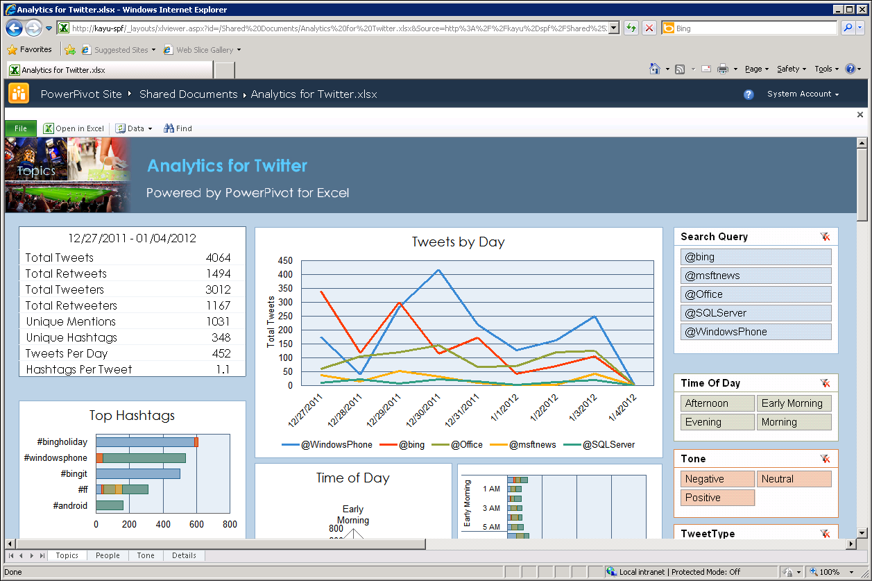
- Save the changes and upload the workbook to SharePoint. Open the workbook in the browser and verify that it provides full interactivity and renders without warnings, as shown in the following screenshot.
Congratulations! This was a serious piece of work, but it was definitely worth it. The Twitter Analytics solution is now a full-blown PowerPivot team application, easily shared through SharePoint and accessible in the browser without the need for Excel 2010 and PowerPivot add-in on the client computer. You can also eliminate the data refresh burden. It was a somewhat complicated and challenging procedure for information workers to refresh the data in the original VSTO version, but now manual refresh is definitely deemphasized. Just configure Scheduled Data Refresh to do this job for you, as illustrated in the following screenshot.
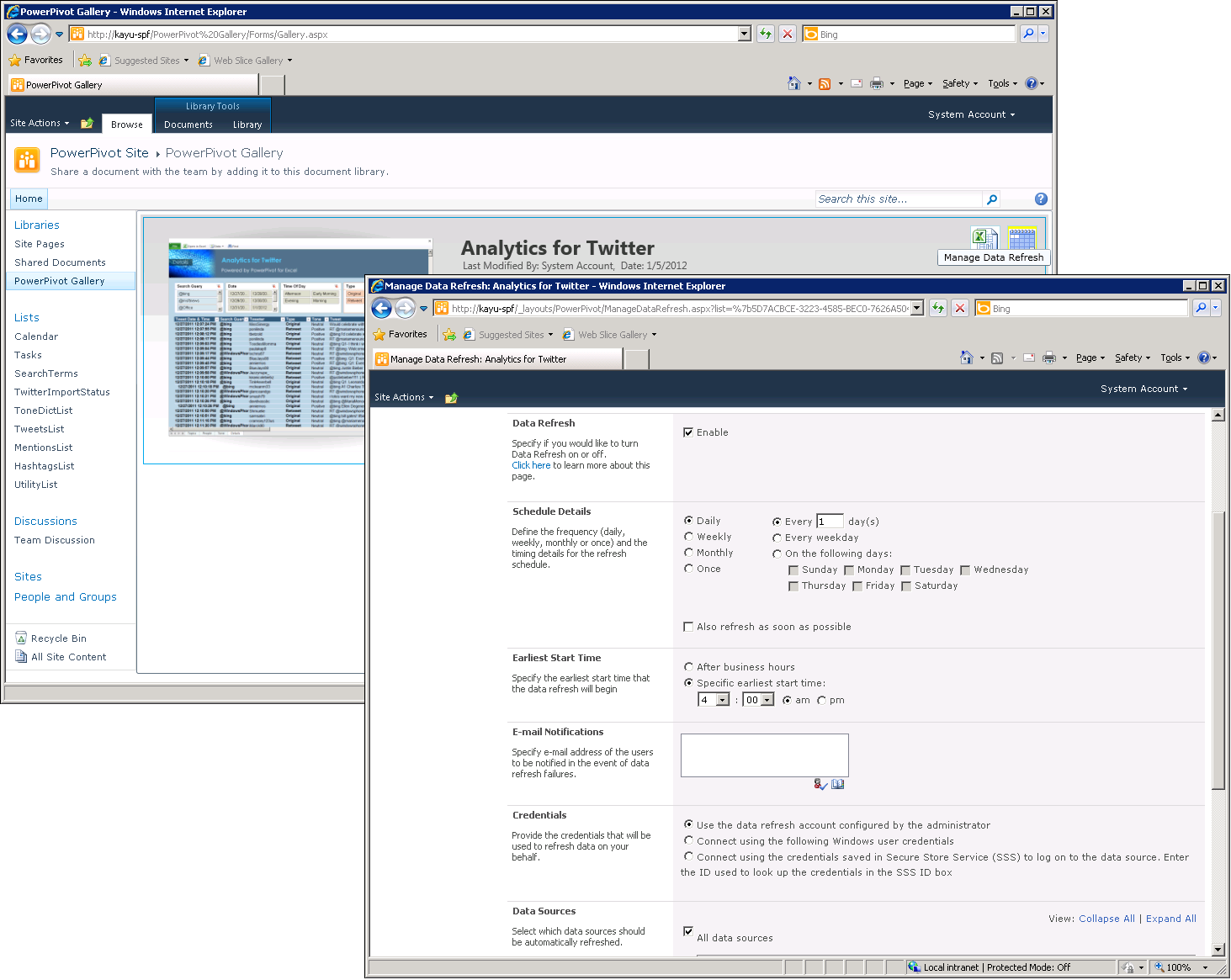
In my test environment, I configured Scheduled Data Refresh to run daily at 4 AM. This was a good choice because my Timer Job tends to finish its import processing around three o’clock every morning according to the Execute Import Job – Finished entries in my TwitterImportStatus list. Refreshing the data during off-business hours after the Twitter Import job finishes ensures that the workbook contains the most recent data when the new workday starts.
And that’s it for now. As demonstrated, you do not necessarily have to use VSTO to build advanced PowerPivot workbooks on top of custom data sources. It can be a valid choice, but in many cases it is worthwhile to look for an alternative import method based on a supported data source. Non-VSTO workbooks are easier to share and can take full advantage of PowerPivot for SharePoint capabilities that are not available to their VSTO counterparts. Admittedly, converting an advanced VSTO workbook, such as the Analytics for Twitter solution, can be a time-consuming effort, especially if you are not the original workbook author, but it’s fortunately not a very common scenario. In any case, I hope you had fun reading this article and following the steps perhaps in your own test environment.