Use DISKSPD to test workload storage performance
Applies to: Azure Stack HCI, versions 22H2 and 21H2; Windows Server 2022, Windows Server 2019
This topic provides guidance on how to use DISKSPD to test workload storage performance. You have an Azure Stack HCI cluster set up, all ready to go. Great, but how do you know if you're getting the promised performance metrics, whether it be latency, throughput, or IOPS? This is when you may want to turn to DISKSPD. After reading this topic, you'll know how to run DISKSPD, understand a subset of parameters, interpret output, and gain a general understanding of the variables that affect workload storage performance.
What is DISKSPD?
DISKSPD is an I/O generating, command-line tool for micro-benchmarking. Great, so what do all these terms mean? Anyone who sets up an Azure Stack HCI cluster or physical server has a reason. It could be to set up a web hosting environment, or run virtual desktops for employees. Whatever the real-world use case may be, you likely want to simulate a test before deploying your actual application. However, testing your application in a real scenario is often difficult – this is where DISKSPD comes in.
DISKSPD is a tool that you can customize to create your own synthetic workloads, and test your application before deployment. The cool thing about the tool is that it gives you the freedom to configure and tweak the parameters to create a specific scenario that resembles your real workload. DISKSPD can give you a glimpse into what your system is capable of before deployment. At its core, DISKSPD simply issues a bunch of read and write operations.
Now you know what DISKSPD is, but when should you use it? DISKSPD has a difficult time emulating complex workloads. But DISKSPD is great when your workload is not closely approximated by a single-threaded file copy, and you need a simple tool that produces acceptable baseline results.
Quick start: install and run DISKSPD
Without further ado, let’s get started:
From your management PC, open PowerShell as an administrator to connect to the target computer that you want to test using DISKSPD, and then type the following command and press Enter.
Enter-PSSession -ComputerName <TARGET_COMPUTER_NAME>In this example, we're running a virtual machine (VM) called “node1.”
To download the DISKSPD tool, type the following commands and press Enter:
$client = new-object System.Net.WebClient$client.DownloadFile("https://github.com/microsoft/diskspd/releases/download/v2.1/DiskSpd.zip","<ENTER_PATH>\DiskSpd-2.1.zip")Use the following command to unzip the downloaded file:
Expand-Archive -LiteralPath <ENTERPATH>\DiskSpd-2.1.zip -DestinationPath C:\DISKSPDChange directory to the DISKSPD directory and locate the appropriate executable file for the Windows operating system that the target computer is running.
In this example, we're using the amd64 version.
Note
You can also download the DISKSPD tool directly from the GitHub repository that contains the open-source code, and a wiki page that details all the parameters and specifications. In the repository, under Releases, select the link to automatically download the ZIP file.
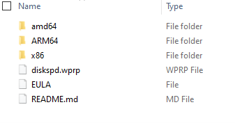
In the ZIP file, you'll see three subfolders: amd64 (64-bit systems), x86 (32-bit systems), and ARM64 (ARM systems). These options enable you to run the tool in every Windows client or server version.
Run DISKSPD with the following PowerShell command. Replace everything inside the square brackets, including the brackets themselves with your appropriate settings.
.\[INSERT_DISKSPD_PATH] [INSERT_SET_OF_PARAMETERS] [INSERT_CSV_PATH_FOR_TEST_FILE] > [INSERT_OUTPUT_FILE.txt]Here is an example command that you can run:
.\diskspd -t2 -o32 -b4k -r4k -w0 -d120 -Sh -D -L -c5G C:\ClusterStorage\test01\targetfile\IO.dat > test01.txtNote
If you do not have a test file, use the -c parameter to create one. If you use this parameter, be sure to include the test file name when you define your path. For example: [INSERT_CSV_PATH_FOR_TEST_FILE] = C:\ClusterStorage\CSV01\IO.dat. In the example command, IO.dat is the test file name, and test01.txt is the DISKSPD output file name.

Specify key parameters
Well, that was simple right? Unfortunately, there is more to it than that. Let’s unpack what we did. First, there are various parameters that you can tinker with and it can get specific. However, we used the following set of baseline parameters:
Note
DISKSPD parameters are case sensitive.
-t2: This indicates the number of threads per target/test file. This number is often based on the number of CPU cores. In this case, two threads were used to stress all of the CPU cores.
-o32: This indicates the number of outstanding I/O requests per target per thread. This is also known as the queue depth, and in this case, 32 were used to stress the CPU.
-b4K: This indicates the block size in bytes, KiB, MiB, or GiB. In this case, 4K block size was used to simulate a random I/O test.
-r4K: This indicates the random I/O aligned to the specified size in bytes, KiB, MiB, Gib, or blocks (Overrides the -s parameter). The common 4K byte size was used to properly align with the block size.
-w0: This specifies the percentage of operations that are write requests (-w0 is equivalent to 100% read). In this case, 0% writes were used for the purpose of a simple test.
-d120: This specifies the duration of the test, not including cool-down or warm-up. The default value is 10 seconds, but we recommend using at least 60 seconds for any serious workload. In this case, 120 seconds were used to minimize any outliers.
-Suw: Disables software and hardware write caching (equivalent to -Sh).
-D: Captures IOPS statistics, such as standard deviation, in intervals of milliseconds (per-thread, per-target).
-L: Measures latency statistics.
-c5g: Sets the sample file size used in the test. It can be set in bytes, KiB, MiB, GiB, or blocks. In this case, a 5 GB target file was used.
For a complete list of parameters, refer to the GitHub repository.
Understand the environment
Performance heavily depends on your environment. So, what is our environment? Our specification involves an Azure Stack HCI cluster with storage pool and Storage Spaces Direct (S2D). More specifically, there are five VMs: DC, node1, node2, node3, and the management node. The cluster itself is a three-node cluster with a three-way mirrored resiliency structure. Therefore, three data copies are maintained. Each “node” in the cluster is a Standard_B2ms VM with a maximum IOPS limit of 1920. Within each node, there are four premium P30 SSD drives with a maximum IOPS limit of 5000. Finally, each SSD drive has 1 TB of memory.
You generate the test file under the unified namespace that the Cluster Shared Volume (CSV) provides (C:\ClusteredStorage) to use the entire pool of drives.
Note
The example environment does not have Hyper-V or a nested virtualization structure.
As you’ll see, it's entirely possible to independently hit either the IOPS or bandwidth ceiling at the VM or drive limit. And so, it is important to understand your VM size and drive type, because both have a maximum IOPS limit and a bandwidth ceiling. This knowledge helps to locate bottlenecks and understand your performance results. To learn more about what size may be appropriate for your workload, see the following resources:
Understand the output
Armed with your understanding of the parameters and environment, you're ready to interpret the output. First, the goal of the earlier test was to max out the IOPS with no regard to latency. This way, you can visually see whether you reach the artificial IOPS limit within Azure. If you want to graphically visualize the total IOPS, use either Windows Admin Center or Task Manager.
The following diagram shows what the DISKSPD process looks like in our example environment. It shows an example of a 1 MiB write operation from a non-coordinator node. The three-way resiliency structure, along with the operation from a non-coordinator node, leads to two network hops, decreasing performance. If you're wondering what a coordinator node is, don’t worry! You'll learn about it in the Things to consider section. The red squares represent the VM and drive bottlenecks.

Now that you've got a visual understanding, let’s examine the four main sections of the .txt file output:
Input settings
This section describes the command you ran, the input parameters, and additional details about the test run.

CPU utilization details
This section highlights information such as the test time, number of threads, number of available processors, and the average utilization of every CPU core during the test. In this case, there are two CPU cores that averaged around 4.67% usage.

Total I/O
This section has three subsections. The first section highlights the overall performance data including both read and write operations. The second and third sections split the read and write operations into separate categories.
In this example, you can see that the total I/O count was 234408 during the 120-second duration. Thus, IOPS = 234408 /120 = 1953.30. The average latency was 32.763 milliseconds, and the throughput was 7.63 MiB/s. From earlier information, we know that the 1953.30 IOPS are near the 1920 IOPS limitation for our Standard_B2ms VM. Don’t believe it? If you rerun this test using different parameters, such as increasing the queue depth, you'll find that the results are still capped at this number.
The last three columns show the standard deviation of IOPS at 17.72 (from -D parameter), the standard deviation of the latency at 20.994 milliseconds (from -L parameter), and the file path.

From the results, you can quickly determine that the cluster configuration is terrible. You can see that it hit the VM limitation of 1920 before the SSD limitation of 5000. If you were limited by the SSD rather than the VM, you could have taken advantage of up to 20000 IOPS (4 drives * 5000) by spanning the test file across multiple drives.
In the end, you need to decide what values are acceptable for your specific workload. The following figure shows some important relationships to help you consider the tradeoffs:

The second relationship in the figure is important, and it's sometimes referred to as Little’s Law. The law introduces the idea that there are three characteristics that govern process behavior and that you only need to change one to influence the other two, and thus the entire process. And so, if you're unhappy with your system’s performance, you have three dimensions of freedom to influence it. Little's Law dictates that in our example, IOPS is the "throughput" (input output operations per second), latency is the "queue time", and queue depth is the "inventory".
Latency percentile analysis
This last section details the percentile latencies per operation type of storage performance from the minimum value to the maximum value.
This section is important because it determines the “quality” of your IOPS. It reveals how many of the I/O operations were able to achieve a certain latency value. It's up to you to decide the acceptable latency for that percentile.
Moreover, the “nines” refer to the number of nines. For example, “3-nines” is equivalent to the 99th percentile. The number of nines exposes how many I/O operations ran at that percentile. Eventually, you'll reach a point where it no longer makes sense to take the latency values seriously. In this case, you can see that the latency values remain constant after “4-nines.” At this point, the latency value is based on only one I/O operation out of the 234408 operations.


Things to consider
Now that you've started using DISKSPD, there are several things to consider to get real-world test results. These include paying close attention to the parameters you set, storage space health and variables, CSV ownership, and the difference between DISKSPD and file copy.
DISKSPD vs. real-world
DISKSPD’s artificial test gives you relatively comparable results for your real workload. However, you need to pay close attention to the parameters you set and whether they match your real scenario. It's important to understand that synthetic workloads will never perfectly represent your application’s real workload during deployment.
Preparation
Before running a DISKSPD test, there are a few recommended actions. These include verifying the health of the storage space, checking your resource usage so that another program doesn't interfere with the test, and preparing performance manager if you want to collect additional data. However, because the goal of this topic is to quickly get DISKSPD running, it doesn't dive into the specifics of these actions. To learn more, see Test Storage Spaces Performance Using Synthetic Workloads in Windows Server.
Variables that affect performance
Storage performance is a delicate thing. Meaning, there are many variables that can affect performance. And so, it's likely you may encounter a number that is inconsistent with your expectations. The following highlights some of the variables that affect performance, although it's not a comprehensive list:
- Network bandwidth
- Resiliency choice
- Storage disk configuration: NVME, SSD, HDD
- I/O buffer
- Cache
- RAID configuration
- Network hops
- Hard drive spindle speeds
CSV ownership
A node is known as a volume owner or the coordinator node (a non-coordinator node would be the node that does not own a specific volume). Every standard volume is assigned a node and the other nodes can access this standard volume through network hops, which results in slower performance (higher latency).
Similarly, a Cluster Shared Volume (CSV) also has an “owner.” However, a CSV is “dynamic” in the sense that it will hop around and change ownership every time you restart the system (RDP). As a result, it’s important to confirm that DISKSPD is run from the coordinator node that owns the CSV. If not, you may need to manually change the CSV ownership.
To confirm CSV ownership:
Check ownership by running the following PowerShell command:
Get-ClusterSharedVolumeIf the CSV ownership is incorrect (For example, you are on Node1 but Node2 owns the CSV), then move the CSV to the correct node by running the following PowerShell command:
Get-ClusterSharedVolume <INSERT_CSV_NAME> | Move-ClusterSharedVolume <INSERT _NODE_NAME>
File copy vs. DISKSPD
Some people believe that they can “test storage performance” by copying and pasting a gigantic file and measuring how long that process takes. The main reason behind this approach is most likely because it's simple and fast. The idea is not wrong in the sense that it tests a specific workload, but it's difficult to categorize this method as “testing storage performance.”
If your real-world goal is to test file copy performance, then this may be a perfectly valid reason to use this method. However, if your goal is to measure storage performance, we recommend to not use this method. You can think of the file copy process as using a different set of “parameters” (such as queue, parallelization, and so on) that is specific to file services.
The following short summary explains why using file copy to measure storage performance may not provide the results that you're looking for:
File copies might not be optimized, There are two levels of parallelism that occur, one internal and the other external. Internally, if the file copy is headed for a remote target, the CopyFileEx engine does apply some parallelization. Externally, there are different ways of invoking the CopyFileEx engine. For example, copies from File Explorer are single threaded, but Robocopy is multi-threaded. For these reasons, it's important to understand whether the implications of the test are what you are looking for.
Every copy has two sides. When you simply copy and paste a file, you may be using two disks: the source disk and the destination disk. If one is slower than the other, you essentially measure the performance of the slower disk. There are other cases where the communication between the source, destination, and the copy engine may affect the performance in unique ways.
To learn more, see Using file copy to measure storage performance.
Experiments and common workloads
This section includes a few other examples, experiments, and workload types.
Confirming the coordinator node
As mentioned previously, if the VM you are currently testing does not own the CSV, you'll see a performance drop (IOPS, throughput, and latency) as opposed to testing it when the node owns the CSV. This is because every time you issue an I/O operation, the system does a network hop to the coordinator node to perform that operation.
For a three-node, three-way mirrored situation, write operations always make a network hop because it needs to store data on all the drives across the three nodes. Therefore, write operations make a network hop regardless. However, if you use a different resiliency structure, this could change.
Here is an example:
- Running on local node: .\DiskSpd-2.0.21a\amd64\diskspd.exe -t4 -o32 -b4k -r4k -w0 -Sh -D -L C:\ClusterStorage\test01\targetfile\IO.dat
- Running on nonlocal node: .\DiskSpd-2.0.21a\amd64\diskspd.exe -t4 -o32 -b4k -r4k -w0 -Sh -D -L C:\ClusterStorage\test01\targetfile\IO.dat
From this example, you can clearly see in the results of the following figure that latency decreased, IOPS increased, and throughput increased when the coordinator node owns the CSV.

Online Transaction Processing (OLTP) workload
Online Transactional Processing (OLTP) workload queries (Update, Insert, Delete) focus on transaction-oriented tasks. Compared to Online Analytical Processing (OLAP), OLTP is storage latency dependent. Because each operation issues little I/O, what you care about is how many operations per second you can sustain.
You can design an OLTP workload test to focus on random, small I/O performance. For these tests, focus on how far you can push the throughput while maintaining acceptable latencies.
The basic design choice for this workload test should at a minimum include:
- 8 KB block size => resembles the page size that SQL Server uses for its data files
- 70% Read, 30% Write => resembles typical OLTP behavior
Online Analytical Processing (OLAP) workload
OLAP workloads focus on data retrieval and analysis, allowing users to perform complex queries to extract multidimensional data. Contrary to OLTP, these workloads are not storage latency sensitive. They emphasize queueing many operations without caring much about bandwidth. As a result, OLAP workloads often result in longer processing times.
You can design an OLAP workload test to focus on sequential, large I/O performance. For these tests, focus on the volume of data processed per second rather than the number of IOPS. Latency requirements are also less important, but this is subjective.
The basic design choice for this workload test should at a minimum include:
512 KB block size => resembles the I/O size when the SQL Server loads a batch of 64 data pages for a table scan by using the read-ahead technique.
1 thread per file => currently, you need to limit your testing to one thread per file as problems may arise in DISKSPD when testing multiple sequential threads. If you use more than one thread, say two, and the -s parameter, the threads will begin non-deterministically to issue I/O operations on top of each other within the same location. This is because they each track their own sequential offset.
There are two “solutions” to resolve this issue:
The first solution involves using the -si parameter. With this parameter, both threads share a single interlocked offset so that the threads cooperatively issue a single sequential pattern of access to the target file. This allows no one point in the file to be operated on more than once. However, because they still do race each other to issue their I/O operation to the queue, the operations may arrive out of order.
This solution works well if one thread becomes CPU limited. You may want to engage a second thread on a second CPU core to deliver more storage I/O to the CPU system to further saturate it.
The second solution involves using the -T<offset>. This allows you to specify the offset size (inter-I/O gap) between I/O operations performed on the same target file by different threads. For example, threads normally start at offset 0, but this specification allows you to distance the two threads so that they will not overlap each other. In any multithreaded environment, the threads will likely be on different portions of the working target, and this is a way of simulating that situation.
Next steps
For more information and detailed examples on optimizing your resiliency settings, see also:
Feedback
Coming soon: Throughout 2024 we will be phasing out GitHub Issues as the feedback mechanism for content and replacing it with a new feedback system. For more information see: https://aka.ms/ContentUserFeedback.
Submit and view feedback for