CNTK Tutorial

• CNTK Tutorial: Getting Started
  • Installing CNTK
  • Logistic Regression
    • Learning Parameters w and b
    • Synthetic Data
    • Setting up Logistic Regression in CNTK
  • Multi-Class Classification
    • Softmax
    • Network Description
    • Putting it all together
• Where to Go Next

CNTK Tutorial: Getting Started

CNTK is a framework for describing learning machines. Although intended for neural networks, the learning machines are arbitrary in that the logic of the machine is described by a series of computational steps in a Computational Network. A Computational Network defines the function to be learned as a directed graph where each leaf node consists of an input value or parameter, and each non-leaf node represents a matrix or tensor operation upon its children. The beauty of CNTK is that once a computational network has been described, all the computation required to learn the network parameters is taken care of automatically. There is no need to derive gradients analytically or to code the interactions between variables for backpropagation.

In this tutorial we will walk through several complete CNTK examples, showing

• how to describe a network in our network-description language BrainScript;
• how to set the learning parameters; and
• how to read in, and write out, data

We will start with a simple implementation of binary classification using the linear model Logistic Regression. From there, we will expand to multiclass classification towards the end of this tutorial. Our next tutorial will tackle a more complex multiclass classification problem that will greatly benefit from a deep network architecture.

The input files (data, scripts) can be found inside the CNTK source-code distribution at Tutorials/HelloWorld-LogisticRegression (GitHub link and can be run directly from there.

Installing CNTK

For the scope of this tutorial it is sufficient to install the CNTK binaries as it is described here.

Logistic Regression

Logistic regression is a simple model for performing binary classification. Given some real-valued d-dimensional example x = (x1 ... xd)', we want to output one of two labels: 0 or 1, true or false, spam or not-spam, etc. So, we want to learn a function y = f(x; w, b) where y is in {0, 1} and w = (w1 ... wd) and b are parameters that we will learn that describe the relationship between x and y.

Like other regression models, logistic regression models the relationship between the independent variable x and the dependent variable z by a linear combination of x with the parameters w and b. In particular, the evidence is described as a linear regression:

z = b + w_1 x_1 + w_2 x_2 + ...

The model learns the weights w and b and determines that, for example, if a high value of x_1 corresponds to a more likely label of y = 1, then the weight w_1 should also be high. If, on the other hand, the value of x_2 corresponds to a more likely label of y = 0, then w_2 should have a large negative value.

The logistic part of logistic regression comes into play because instead of predicting an unbounded number, we are instead interested in predicting the probability of one of two labels. To output a probability, we transform the evidence using the logistic function: sigma(x) = 1 / (1 + exp(-x)). The logistic function looks like this:

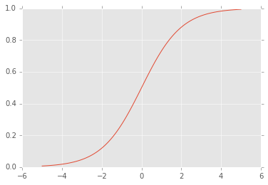
So, applying the logistic function has the effect of 'squashing' the evidence to fall between 0 and 1. Large positive evidence values become close to 1, and large negative evidence values become close to 0. This allows our model to output probabilities.

Our model can then be seen as y ~ p(y | x; w, b) = sigma(wx+b) = 1 / (1 + exp(-wx-b)) Then, we predict y = 1 if p(y | x; w, b) > 0.5 and y = 0 otherwise.

Learning Parameters w and b

Without CNTK, we need to choose an optimization procedure and solve the derivatives of a cost function with respect to the parameters we want to learn. Seeing logistic regression as a probabilistic model, we can maximize the likelihood of the data. This turns out to be the same as minimizing the cross-entropy cost function, which for logistic regression is also known as the 'logistic loss function'. In general this cannot be done analytically, but we can determine analytic solutions for the gradients and then use gradient descent to converge towards the correct parameters.

CNTK uses the common stochastic gradient descent (SGD) algorithm to learn parameters in a Computational Network. The gradients are determined through automatic differentiation. Before going through how we would set up the problem in CNTK, let's take a look at the data we will use for our first classification problem.

Synthetic Data

We will start with an easy, but visualizable problem. This data is generated by sampling from two 2-dimensional gaussians with different means. The script used to generate the data is here and pre-generated data from this script is included for training and testing. Plotting the training data looks like this:

Our task is to classify and point in the 2D plane as originating from one of the two classes. As we said, it's an easy problem to start with :-)

Setting up Logistic Regression in CNTK

To setup and train the Computational Network, we will write a .cntk configuration file that

1. describes the network;
2. specifies the commands we want to perform on the network (train, test, output, etc.);
3. sets how we want to learn the parameters of the network (SGD and its parameters); and
4. how CNTK should read and write the data.

We will start with how to describe the Computational Network.

Describing Logistic Regression as a Computational Network

To describe our Computational Network, we use CNTK's network-description language BrainScript. We will need to define:

• the input features
• the labels
• the parameters to learn
• the computational operations, and
• the root nodes (outputs)

Let's go through them each in turn. First, though, here is the .cntk block that describes our network:

BrainScriptNetworkBuilder = {

    # sample and label dimensions
    SDim = $dimension$      defined as 2 outside
    LDim = 1

    features = Input {SDim}
    labels   = Input {LDim}

    # parameters to learn
    b = ParameterTensor {LDim}         # bias
    w = ParameterTensor {(LDim:SDim)}  # weights

    # operations
    p = Sigmoid (w * features + b)    

    lr = Logistic (labels, p)
    err = SquareError (labels, p)

    # root nodes
    featureNodes    = (features)
    labelNodes      = (labels)
    criterionNodes  = (lr)
    evaluationNodes = (err)
    outputNodes     = (p)
}

Input features and labels

The two principal inputs to the network are the features and the labels. Because we have two-dimensional data, we set the features to be of type Input{} where the dimension of a sample is 2. All objects are matrices so we defined a single sample of our features to be a matrix with SDim (2) rows and 1 column.

We must also define the possible labels. Because we are performing binary classification, we could set this up either as a multi-class classification problem where we will predict the probability of label 0 and the probability of label 1, or we can see the problem as the equivalent true binary classification problem that only wants to predict one of the labels. In the latter case, the probability of the other label is of course p(y=0) = 1 - p(y=1). In this tutorial we match the original definition of LR and go with the one label prediction.

Model parameters

Above we defined the evidence for logistic regression as

z = b + w_1 x_1 + w_2 x_2 + ...

Because our input data has 2 dimensions, and we are only predicting a single label, w will be a row vector (expressed as a [1 x 2] matrix) and b will be a scalar value (expressed as a [1 x 1] matrix).

Computational operations

Next we need to express the logistic-regression function. This is straight-forward in BrainScript:

p = Sigmoid (w * features + b)

Under the hood, this will expand into these 3 successive operations as nodes in the graph:

1. multiply the weights w with the features,
2. add the bias term b, and
3. squash the evidence down to a probability p.

Next, we want to describe the criteria that are used to learn the parameters. The line

lr = Logistic (labels, p)

sets up a criterion node that is used for learning the parameters that are involved in any related computation. Here, we are specifying that CNTK should run the Logistic loss function with the correct answers labels and the current predictions p. The function Logistic() is built-in to CNTK and computes the loss for each sample as -(l' log(p) + (1-l)' log(1-p)), where l denotes the one-hot label vector for the sample, log() is taken element-wise, and ' indicates transposition.

In fact, it is possible to write your own loss function. For example, the above logistic loss can be written directly in the configuration file:

lr = -(TransposeTimes (labels, Log (p)) +
       TransposeTimes (Constant(1) - labels, Log (Constant(1) - p)))

The lines

err = SquareError (labels, p)
evaluationNodes = (err)

allow for model evaluation as the training occurs. In addition to the criterionNodes, evaluationNodes are computed and logged during training: While the learning is solely concerned with minimizing the logistic loss, in the end we are actually (probably) most interested in accuracy. We can then evaluate the model as it trains by setting up an evaluation node as we do here. Often, accuracy is measured differently from training loss. In the above example, we use the square error as an accuracy measurement. For multi-class classification tasks with 3 or more classes, we would normally use the classification error for model evaluation.

Root nodes

Finally, we describe the root nodes of the network. This section is for specifying some special nodes that have a particular meaning in CNTK. For example, the criterionNodes are those where an objective is specified that CNTK will try to achieve, the evaluationNodes are the nodes used for perfoming evaluation as the model is trained, and the outputNodes are the nodes whose values will be output. This final node is important because these are the actual values that the model is predicting for a given input. Again, this node is optional but useful for seeing how the model is performing on its ultimate goal.

Specifying the commands to run

Let us now look at the other aspects of the .cntk file. A .cntk file consists of variable assignments of the form parameterVariable = parameterValue.

An important parameter in the .cntk file is command, which specifies the operations that CNTK should execute. These operations are specified by the user and defined in the configuration file. Our example includes the following:

command=Train:Output:DumpNodeInfo:Test

Each of the commands is separated by a : and you can have as many commands as you require for your particular use case. Commands are simply a way to organize functions of your network, and the CNTK 'program' will just execute them one by one. Let's go through the Train command with the details hidden away.

Command Train

# training config
Train = {             # command=Train --> CNTK will look for a parameter named Train
    action = "train"  # execute CNTK's 'train' routine

    # network description
    BrainScriptNetworkBuilder = {
        ...
    }

    # configuration parameters of the SGD procedure
    SGD = {
        ...
    }

    # configuration of data reading
    reader = {
        ...
    }
}

We first specify that the action of this command is to "train". The action parameter selects one of several pre-defined CNTK procedures to be executed. (There is, however, nothing special about the command name "Train" itself.) The Train command has three major components that must be configured:

• our network (as discussed in the previous section),
• how to learn on the computational network with the SGD Learner (next section),
• and the reader that will import our training data into the network (section below on Data Readers).

Command Output

The Output command is defined in our CNTK configuration file as follows:

# output the results
Output = {
    action = "write"
    reader = {
        readerType = "CNTKTextFormatReader"
        file = "Test_cntk_text.txt"
        input = {
            features = { dim = $dimension$ ; format = "dense" }  # $$ means variable substitution
            labels   = { dim = 1           ; format = "dense" }
        }
    }
    outputPath = "LR.txt"  # dump the output to this text file
}

Again, there is nothing special about the name Output, while the action parameter selects the CNTK write procedure, which has the purpose of applying a network to data read, writing the output(s) to a file. For that, we specify the reader (details explained below) and the outputPath. The outputPath gives the prefix for the file that will be written; the actual file will have the name of the output variable appended to the end.

So, what does this output? The values written are the probabilities that a sample belongs to class 1. This is our variable p, which was declared an output with outputNodes = (p)). Our Output command will read in our test data "Test_cntk_text.txt", run it through the learned model, and output the values for each of the examples into the file "LR.txt.p".

Command Test

The Test command performs the action test. It will compute the values of specified evaluationNodes from our network description. Just as above with the Output command, we will specify a reader for some test data. However, unlike Output which simply wrote the prediction probabilities for each test sample to file, it will compute the specified error metric for the test set. In our example, that is the function SquareError() as specified in the configuration. Here is the description of the Test command:

Test = {
    action = "test"
    reader = {
        readerType = "CNTKTextFormatReader"
        file = "Test_cntk_text.txt"
        input = {
            features = { dim = $dimension$ ; format = "dense" }
            labels   = { dim = 1           ; format = "dense" }
        }
    }
}

While Logistic measured the training loss and guided the model parameter updates, we use SquareError to measure the classification error after each iteration on the test set (this might normally be done with a separate validation set). It takes the matrix p, which is the prediction probability for class 1 of our model, and compares it to the correct labels. The final output will give the error per sample of our network on the test/validation data.

Remember that in our CNTK configuration file it looks like this:

err = SquareError (labels, p)
evaluationNodes = (err)

Command DumpNodeInfo

The DumpNodeInfo command in our example is defined as follows:

DumpNodeInfo = {
    action = "dumpNode"
    printValues = true
}

This command simply outputs all model parameters in the network. This can be useful for debugging and for doing further processing with what your network learned. For example, for the synthetic data described above, CNTK will learn the parameters w and the bias b. We can use CNTK to perform prediction on a test set (as described below), but we might also be interested in visualizing what decision boundary is described by our model. Let's do that here.

The DumpNodeInfo command outputs a file called "LR.dnn.__AllNodes__.txt" into the Models directory. Following the training of our example, that file contains, in addition to lines that represent the model structure, the values of the parameters w and b:

b=LearnableParameter [1,1]   learningRateMultiplier=1.000000  NeedsGradient=true
 -12.3975668
w=LearnableParameter [1,2]   learningRateMultiplier=1.000000  NeedsGradient=true
 2.40208364 2.66412568

Let's see how this translates to our decision boundary. Our evidence is z = b + x_1 w_1 + x_2 w_2. If z > 0, which is the same as p = sigma(z) > 0.5, then we predict y = 1. If z < 0, we predict y = 0. Therefore, our decision boundary occurs when z = 0. Then,

0 = b + x_1 w_1 + x_2 w_2

x_2 = -x_1 (w_1 / w_2) - (b / w_2)

The above is just the standard equation of a line y = mx + a with y = x_2 and x = x_1, the slope m = (-w_1 / w_2), and the bias a = -b / w_2. If we then plug in the values from "LR.dnn.__AllNodes__.txt", b = -12.3975668, w_1 = 2.40208364, and w_2 = 2.66412568, we see:

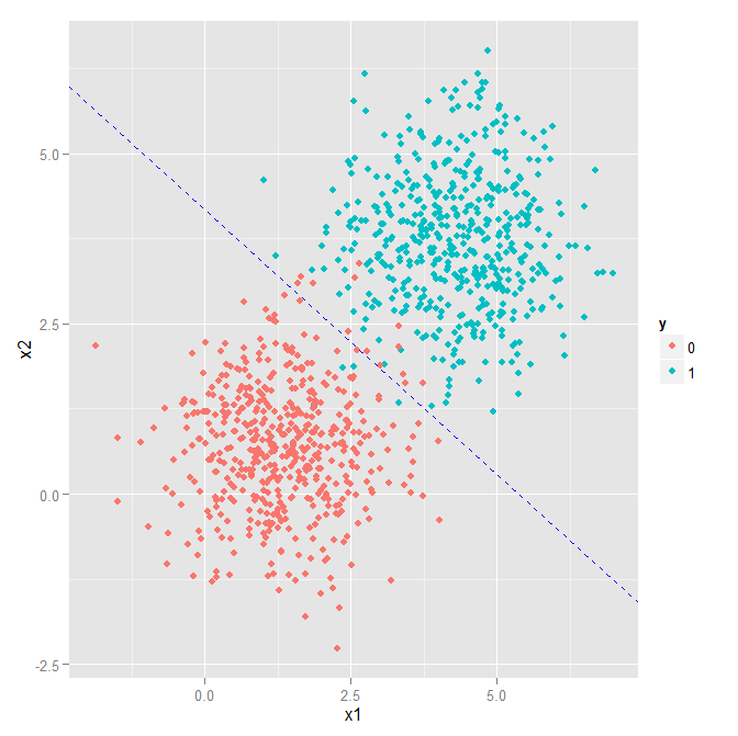
Not bad!

Setting up the learning algorithm

Finally, to be able to learn the parameters that we used above, CNTK needs to make use of a learning algorithm. That algorithm is stochastic gradient descent (SGD). SGD iteratively looks at some fixed subset of the training examples (called a minibatch) and updates the parameters in the direction of the cost function gradients after every such step, such that if it was to see the same data again, the network output would be a little closer to the desired result.

Optimizing parameters for neural nets is in general not a convex optimization problem, so for all but the simplest cases there is not a single global optimum. By looking at a minibatch instead of the full data, every update follows just a rough approximation of the final training target. SGDs "stochastic" nature helps jumping out of local optima and has proven to be both simple and effective for finding good solutions. Using CNTK's implementation of SGD allows a number of settings to fit the problem at hand. For our simple problem, we set up SGD in the .cntk file as follows:

SGD = {
    epochSize = 0
    maxEpochs = 50
    minibatchSize = 25
    learningRatesPerSample = 0.04
}

The epochSize determines how many examples will be examined per epoch. If it is set to 0 then that means all of the training data will be examined for every epoch (also can be thought of as iteration). Within each iteration, minibatches of samples (in this case 25) are examined together and their gradients are computed. At the end of the mini-batch, the sum over all 25 gradients is used to alter the parameters.

The learningRatesPerSample gives the SGD learning rate. This controls how big of a step to take in the direction of the gradient for each parameter update. Here, we use a constant learning rate of 0.04, which means that every gradient contributes by being weighted with 0.04 and then subtracted from the model parameters.

CNTK also allows to specify a learning-rate profile over epochs (typically a descending learning rate) by providing multiple values separated by a :. Finally, values can be repeated over multiple epochs by using *. For example:

learningRatesPerSample = 0.05:0.02*5:0.01

is the same as writing

learningRatesPerSample = 0.05:0.02:0.02:0.02:0.02:0.02:0.01

and will slowly descend the learning rate per mini batch until it settles at 0.01.

Note that CNTK differs from other toolkits in that it uses the sum over sample gradients, while other toolkits may use the average. If the learning rate is specified by the alternate parameter learningRatesPerMB, it will be divided by the specified MB size, emulating averaging behavior.

Finally, maxEpochs gives the maximum number of epochs to perform before terminating the algorithm. In this case, we will run SGD for exactly 50 epochs because there are no other stopping criteria specified. CNTK allows to specify early stopping criteria that would stop learning once the error reaches some threshold. CNTK also supports other forms of early stopping, momentum (don't diverge too far from a previous update's direction), and other advanced gradient descent features. They will be covered in a later tutorial.

How to read and write data (Data Readers)

Reading and writing data is performed using Data Readers. A reader is defined as a sub-block in the configuration file, within a command. The following reader definition is the one used in our example:

reader = {
    readerType = "CNTKTextFormatReader"
    file = "Train_cntk_text.txt"
    input = {
        features = { dim = 2 ; format = "dense" }
        labels   = { dim = 1 ; format = "dense" }
    }
}

In our example we use the following parameters:

• readerType: In our example we will use CNTKTextFormatReader, which is designed to read the text-based CNTK format, described in detail on this page.
• file: the file that contains the dataset
• dim: the dimension of the input vector.
• format: the type of the input vector, can be dense or sparse.

Among other things, this particular reader supports grouping lines into variable length sequences and, for example, it can be used to set up RNN training. Please check the reader documentation for additional info.

Putting it all together

In the previous several sections, we have explained how to describe the computational network, how to read in data, and how to setup the learning that will be done over the network. Here, let's put it all together into a single CNTK configuration file.

The final configuration file is here. (Also ensure that Test_cntk_text and Train_cntk_text files are present in your working directory.) The order of defining commands is not important. For example, we can have command=Train:Test and then define Test first, followed by Train. What matters is the order of the commands within the command= line.

In our CNTK configuration file, the first line reads command=Train:Output:DumpNodeInfo:Test. So, when we run it through CNTK we will train the model, output the predictions, dump the node info, and finally test the network. For all of this magic to happen, we simply run:

cntk  configFile=lr_bs.cntk

or, if you are self-compiling under Windows, you can run this from inside Visual Studio with these Debugging Command Arguments:

currentDirectory=$(SolutionDir)Examples\Tutorial  configFile=lr_bs.cntk

And that's it! You have now successfully defined a computational network that performs binary classification, learned the parameters, and tested its accuracy. Here is the end of the output from running the above command:

Final Results: Minibatch[1-1]: err = 0.00688694 * 500
COMPLETED!

So on our test data (as we would expect given the decision boundary we plotted above), we did quite well. This is about as good as we can possibly do given that the classes slightly overlap.

Using the GPU

The example so far has been described to use CNTK in CPU mode only. To make use of the GPU, which is typically an order of magnitude faster, the deviceId parameter must be set. This can be done within the .cntk file, or at the command line as follows:

cntk  configFile=lr_ndl.cntk  deviceId=auto

This will make CNTK use the GPU for computation. See more on the deviceId parameter here (Windows) or here (Linux).

This shows an important mechanism: Any key-value pair on the command-line parameter of the CNTK executable "patches" an existing configuration (with the exception of the key "configFile" which is always required to set a "base" configuration). Thus, the above is equivalent to having a deviceId key in the file itself.

Now let's make things a little more interesting with multi-class classification...

Checkpointing and makeMode

After each epoch, CNTK will write a checkpoint file that allows to restart training in case it gets interrupted. This is controlled through the top-level configuration variable makeMode which defaults to true.

This is the reason that if you run the above command line twice, the second time it will not repeat the training--since CNTK has discovered that all epochs have already been completed. To run the sample multiple times from scratch, override makeMode, for example:

cntk  configFile=lr_bs.cntk  makeMode=false

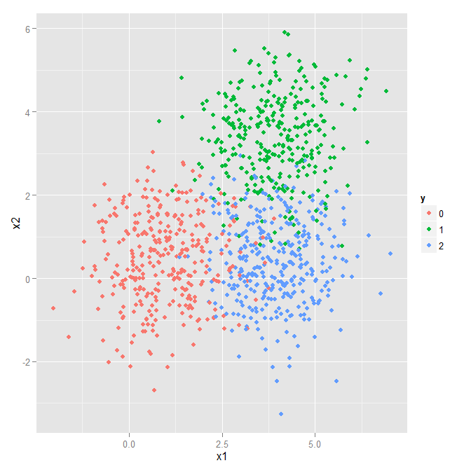
Multi-Class Classification

Let us make our simple problem slightly harder by adding a third class. We can borrow the majority of what we used for the binary classification problem above. However, when using more than two output classes, we must use the softmax function instead of the sigmoid. So, let us start with a quick introduction of the softmax before building the computational network for this problem.

Softmax

The softmax function is a generalization of the logistic function. It maps a vector of real values to a probability distribution. It is widely used for multi-class classification problems. In this context, if we are trying to predict the class of an instance out of K possible classes, the model would compute a K-dimensional vector whose components represent the confidence scores for each class. Then, the softmax function would map those scores to a posterior probability distribution over the possible classes using the following formula:

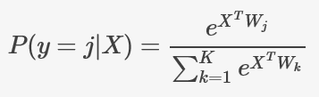
where X is our input vector, and W is the weight matrix, that includes both the model parameters and the bias.

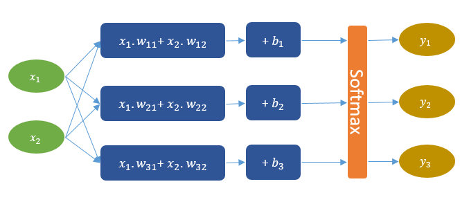
Network Description

We want to define a computational network that looks like the one in the figure below. This network can be understood as a combination of three linear models, each of which will be trained to separate one of the three classes from the other two. Then, on top, we have the softmax layer that squashes the linear model scores into a probability distribution. Thus, for each instance, the network outputs three probability values that sum up to one. For example, if a given instance is of class (1), the model might output the following probabilities (95%, 3%, 2%), which basically means that the probability of the instance belonging to class (1) is 95%.

Armed with what we have already learned about CNTK's network builder, let's build the network that solves our 3-class problem. Actually, we are already almost done, as such a network is very similar to the one we already used for our binary classification problem, but with a few differences:

• the label dimension is now 3 instead of 1;
• we take out the Sigmoid() node;
• we replace the Logistic() learning criterion by CrossEntropyWithSoftmax() which will add the softmax layer and use cross entropy as the objective function; and
• we replaced the SquareError() evaluation node with ErrorPrediction().

Here's our new network:

BrainScriptNetworkBuilder=[

    # sample and label dimensions
    SDim = $dimension$      # defined as 2 outside
    LDim = $labelDimension$ # defined as 3 outside

    features = Input {SDim}
    labels   = Input {LDim}

    # parameters to learn
    b = ParameterTensor {LDim}
    w = ParameterTensor {(LDim:SDim)}

    # operations
    z = w * features + b

    ce = CrossEntropyWithSoftmax (labels, z)
    errs = ErrorPrediction (labels, z)

    # root nodes
    featureNodes    = (features)
    labelNodes      = (labels)
    criterionNodes  = (ce)
    evaluationNodes = (errs)
    outputNodes     = (z)
]

Putting it all together

Similarly to the binary classification problem, the final configuration file is here together with Test and Train sets. We run:

cntk  configFile=3Classes_bs.cntk

(This will run CNTK on CPU - see more on this in the previous section)

And that's it! You have now successfully defined a computational network that performs multi-class classification, learned the parameters, and tested it. Here is the end of the output from running the above command:

Final Results: Minibatch[1-1]: errs = 10.200% * 500; ce = 0.24347000 * 500; perplexity = 1.27566805
COMPLETED!

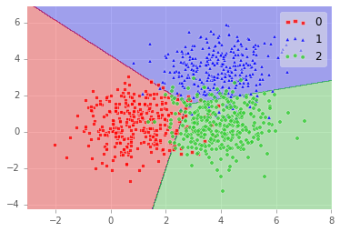
So on our test data (as we would expect given the decision boundary we plotted below), we did well: 89.8% accuracy!

Where To Go Next

Check out Tutorial II to learn how to build more complex models like convolutional neural networks.