Tutorial: Data import and exploration using RevoScaleR
Important
This content is being retired and may not be updated in the future. The support for Machine Learning Server will end on July 1, 2022. For more information, see What's happening to Machine Learning Server?
Applies to: Microsoft R Client, Machine Learning Server
In data-driven projects, one action item guaranteed to be on the list is data acquisition and exploration. In this tutorial, you will learn how to import a text-delimited .csv file into an R session and use functions from RevoScaleR to ascertain the shape of the data.
To load data, use rxImport from the RevoScaleR function library. The rxImport function converts source data into a columnar format for consumption in R and returns a data source object that wraps a dataset with useful metadata. Optionally, by specifying an outFile parameter, you can create an XDF file if you want to persist the data for future calculations.
Note
R Client and Machine Learning Server are interchangeable in terms of RevoScaleR as long as data fits into memory and processing is single-threaded. If datasets exceed memory, we recommend pushing the compute context to Machine Learning Server.
What you will learn
- How to load CSV data using rxImport and optionally save it as an XDF
- How to obtain information about the data structure
- Use parameters for selective import and conversion
- Summarize data
- Subset and transform data
Prerequisites
To complete this tutorial as written, use an R console application and built-in data.
- On Windows, go to \Program Files\Microsoft\R Client\R_SERVER\bin\x64 and double-click Rgui.exe.
- On Linux, at the command prompt, type Revo64.
The command prompt for R is >. You can hand-type case-sensitive R commands, or copy-paste multi-line commands at the console command prompt. The R interpreter can queue up multiple commands and run them sequentially.
How to locate built-in data
RevoScaleR provides both functions and built-in datasets, including the AirlineDemoSmall.csv file used in this tutorial. The sample data directory is registered with RevoScaleR. Its location can be returned through a "sampleDataDir" parameter on the rxGetOption function.
Open the R console or start a Revo64 session. The RevoScaleR library is loaded automatically.
Retrieve the list of sample data files provided in RevoScaleR by entering the following command at the
>command prompt:list.files(rxGetOption("sampleDataDir"))
The open-source R list.files command returns a file list provided by the RevoScaleR rxGetOption function and the sampleDataDir argument.
Note
If you are a Windows user and new to R, be aware that R script is case-sensitive. If you mistype rxGetOption or sampleDataDir, you will get an error instead of the file list.
How to locate the working directory
Both R and RevoScaleR use the working directory to store any files that you create. The following open-source R command provides the working directory location: getwd().
Depending on your environment, you might not have permission to save files to this directory. On Windows, if the output is something like C:/Program Files/Microsoft/ML Server/R_SERVER/bin/x64, you won't have write permissions on that older. To change the working directory, run setwd("C:/Users/TEMP").
Alternatively, specify a fully-qualified path to a writable directory whenever a file name is required (for example, outFile="C:/users/temp/airExample.xdf" on an rxImport call).
Windows users, please note the direction of the path delimiter. By default, R script uses forward slashes as path delimiters.
About the airline dataset
The AirlineDemoSmall.csv dataset is used in this tutorial. It's a subset of a larger dataset containing information on flight arrival and departure details for all commercial flights within the USA, from October 1987 to April 2008. The file contains three columns of data: ArrDelay, CRSDepTime, and DayOfWeek, with a total of 600,000 rows.
Load data
As a first step, perform a preliminary import using the airline data. Initially, the data is loaded as a data frame that exists only in memory.
	mysource <- file.path(rxGetOption("sampleDataDir"), "AirlineDemoSmall.csv")
	airXdfData <- rxImport(inData=mysource)
On the first line,mysource is an object specifying source data created using R's file.path command. The folder path is provided through RevoScaleR's rxGetOption("sampleDataDir"), with "AirlineDemoSmall.csv" for the file.
On line two, airXdfData is a data source object returned by rxImport, which we can query to learn about data characteristics.
Save as XDF
Although we could work with the data frame for the duration of the session, it often helps to save the data as an .xdf file for reuse at a later date. To create an .xdf file, run rxImport with an outFile parameter specifying the name and a folder for which you have write permissions:
airXdfData <- rxImport(inData=mysource, outFile="c:/Users/Temp/airExample.xdf")
Common errors occurring on your first file save exercise might include:
- "Error: '\u' used without hex digits in character string..." indicates an invalid path delimiter. R uses forward slash delimiters (/), even if the path is on the Windows file system.
- "Error in file <>; Permission denied" is obviously a permission error. Choosing a different folder or granting write-access to the current folder will resolve the error.
About data storage in Machine Learning Server
In Machine Learning Server, you can work with in-memory data as a data frame, or save it to disk as an XDF file. As noted, rxImport can create a data source object with or without the .xdf file. If you omit the outFile argument or set it NULL, the return object is a data frame containing the data.
A data frame is the fundamental data structure in R and is fully supported in Machine Learning Server. It is tabular, composed of rows and columns, where columns contain variables and the first row, called the header, stores column names. Subsequent rows provide data values for each variable associated with a single observation. A data frame is a temporary data structure, created when you load some data. It exists only for the duration of the session.
An .xdf file is a binary file format native to Machine Learning Server, used for persisting data on disk. The organization of an .xdf file is column-based, one column per variable, which is optimum for the variable orientation of data used in statistics and predictive analytics. With .xdf, you can load subsets of the data for targeted analysis. Also, .xdf files include precomputed metadata that is immediately available with no additional processing.
Creating an .xdf is not required, but when datasets are large or complex, .xdf files can help by compressing data and by allocating data into chunks that can be read and refreshed independently. Additionally, on distributed file systems like Hadoop's HDFS, XDF files can store data in multiple physical files to accommodate very large datasets.
Tip
You can use rxImport to load all or part of an .xdf into a data frame by specifying an .xdf file as the input. Doing so instantiates a data source object for the .xdf file, but without loading its data. Having an object represent the data source can come in handy. It doesn’t take up much memory, and it can be used in many other RevoScaleR objects interchangeably with a data frame.
Examine object metadata
You should now have a mysource object and an airXdfData object representing the data source. Once a data source object exists, you can use the rxGetInfo function to return metadata and learn more about the structure. Adding the getVarInfo argument returns metadata about variables:
rxGetInfo(airXdfData, getVarInfo = TRUE)
Notice how the output includes the precomputed metadata for each variable, plus a summary of observations, variables, blocks, and compression information. Variables are based on fields in the CSV file. In this case, there are 3 variables.
File name: C:\Users\TEMP\airExample.xdf
Number of observations: 6e+05
Number of variables: 3
Number of blocks: 2
Compression type: zlib
Variable information:
Var 1: ArrDelay, Type: character
Var 2: CRSDepTime, Type: numeric, Storage: float32, Low/High: (0.0167, 23.9833)
Var 3: DayOfWeek, Type: character
From the output, we can determine whether the number of observations is large enough to warrant subdivision into smaller blocks. Additionally, we can see which variables exist, the data type, and for numeric data, the range of values. The presence of string variables is a consideration. To use this data in subsequent analysis, we might need to convert strings to numeric data for ArrDelay. Likewise, we might want to convert DayOfWeek to a factor variable so that we can group observations by day. We can do all of these things in a subsequent import.
Tip
To get just the variable information, use the standalone rxGetVarInfo() function to return precomputed metadata about variables in the .xdf file (for example, rxGetVarInfo(airXdfData)).
Convert on re-import
The rxImport function takes multiple parameters that can be used to modify data during import. In this exercise, repeat the import and change the dataset at the same time. By adding parameters to rxImport, you can:
- Convert the string column, DayOfWeek, to a factor variable using the stringsAsFactors argument.
- Convert missing values to a specific value, such as the letter M rather than the default NA.
- Allocate rows into blocks that you can subsequently read and write in chunks. By specifying the argument rowsPerRead, you can read and write the data in 3 blocks of 200,000 rows each.
	airXdfData <- rxImport(inData=mysource, outFile="c:/Users/Temp/airExample.xdf",
	stringsAsFactors=TRUE, missingValueString="M", rowsPerRead=200000,
    overwrite=TRUE)
Running this command refreshes the airXdfData data source object. Metadata for the new object reflects the allocation of rows among 3 blocks and conversion of string-to-numeric data for both ArrDelay and DayOfWeek.
> rxGetInfo(airXdfData)
Variable information:
Var 1: ArrDelay
		702 factor levels: 6 -8 -2 1 -14 ... 451 430 597 513 432
Var 2: CRSDepTime, Type: numeric, Storage: float32, Low/High: (0.0167, 23.9833)
Var 3: DayOfWeek
		7 factor levels: Monday Tuesday Wednesday Thursday Friday Saturday Sunday
Control string conversion and factor level ordering
Setting stringsAsFactors to TRUE has built-in behaviors that can have unintended consequences. For example, we might not want every character variable to become a factor. In the case of ArrDelay, the data is actually numeric. You can use the colClasses argument to explicitly set the data type of a particular variable.
Additionally, factor levels are listed arbitrarily in the order in which they are encountered during import, which might not make sense. To override the default, you can explicitly specify the levels in a predefined order using the colInfo argument.
Rerun the import operation to use a fixed data type for ArrDelay and a fixed order for days of the week:
colInfo <- list(DayOfWeek = list(type = "factor",
	levels = c("Monday", "Tuesday", "Wednesday", "Thursday", "Friday", "Saturday", "Sunday")))

airXdfData <- rxImport(inData=mysource, outFile="c:/Users/Temp/airExample.xdf", missingValueString="M",
rowsPerRead=200000, colInfo  = colInfo, colClasses=c(ArrDelay="integer"),
overwrite=TRUE)
Notice that once you supply the colInfo argument, you no longer need to specify stringsAsFactors because DayOfWeek is the only factor variable.
Visualize data
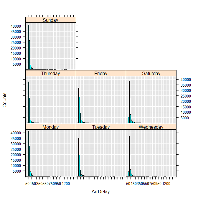
To get a sense of data shape, use the rxHistogram function to show the distribution in arrival delay by day of week. Internally, this function uses the rxCube function to calculate information for a histogram:
rxHistogram(~ArrDelay|DayOfWeek, data = airXdfData)
You can also compute descriptive statistics for the variable:
	rxSummary(~ ArrDelay, data = airXdfData)

		Call:
		rxSummary(formula = ~ArrDelay, data = airXdfData)

		Summary Statistics Results for: ~ArrDelay
		Data: airXdfData (RxXdfData Data Source)
		File name: airExample.xdf
		Number of valid observations: 6e+05

		Name     Mean     StdDev   Min Max  ValidObs MissingObs
		ArrDelay 11.31794 40.68854 -86 1490 582628   17372
Create a new variable
This first look at the data tells us two important things: arrival delay has a long “tail” for every day of the week, with a few flights delayed for well over two hours, and there are quite a few missing values (17,372). Presumably the missing values for arrival delay represent flights that never arrived and thus canceled.
You can use RevoScaleR’s data step functionality to create a new variable, VeryLate, that represents flights that were either over two hours late or canceled. Because the original data is safely preserved in the original text file, we can simply add this variable to our existing XDF file using the transforms argument to rxDataStep. The transforms argument takes a list of one or more R expressions, typically in the form of assignment statements. In this case, we use the following expression: list(VeryLate = (ArrDelay > 120 | is.na(ArrDelay))
The full RevoScaleR data step consists of the following steps:
Read in the data a block (200,000 rows) at a time.
For each block, pass the ArrDelay data to the R interpreter for processing the transformation to create VeryLate.
Write the data out to the dataset a block at a time. The argument overwrite=TRUE allows us to overwrite the data file.
airXdfData <- rxDataStep(inData = airXdfData, outFile = "c:/Users/Temp/airExample.xdf",
	transforms=list(VeryLate = (ArrDelay > 120 | is.na(ArrDelay))),
	overwrite = TRUE)
Output from this command reflects the creation of the new variable:
> rxGetInfo(airXdfData, getVarInfo = TRUE)
File name: C:\Users\TEMP\airExample.xdf
Number of observations: 6e+05
Number of variables: 4
Number of blocks: 3
Compression type: zlib
Variable information:
Var 1: ArrDelay, Type: integer, Low/High: (-86, 1490)
Var 2: CRSDepTime, Type: numeric, Storage: float32, Low/High: (0.0167, 23.9833)
Var 3: DayOfWeek
	7 factor levels: Monday Tuesday Wednesday Thursday Friday Saturday Sunday
Var 4: VeryLate, Type: logical, Low/High: (0, 1)
Summarize data
We already used rxSummary to get an initial impression of data shape, but let's take a closer look at its arguments. The rxSummary function takes a formula as its first argument, and the name of the dataset as the second. To get summary statistics for all of the data in your data file, you can alternatively use the R summary method for the airXdfData object.
> rxSummary(~ArrDelay+CRSDepTime+DayOfWeek, data=airXdfData)
or
> summary(airXdfData)
Summary statistics will be computed on the variables in the formula. By default, rxSummary computes data summaries term-by-term, and missing values are omitted on a term-by-term basis.
Call:
rxSummary(formula = ~ArrDelay + CRSDepTime + DayOfWeek, data = airDS)

Summary Statistics Results for: ~ArrDelay + CRSDepTime + DayOfWeek
Data: airXdfData (RxXdfData Data Source)
File name: C:\Users\TEMP\airExample.xdf
Number of valid observations: 6e+05

	Name       Mean     StdDev    Min        Max        ValidObs MissingObs
	ArrDelay   11.31794 40.688536 -86.000000 1490.00000 582628   17372
	CRSDepTime 13.48227  4.697566   0.016667   23.98333 600000       0

Category Counts for DayOfWeek
Number of categories: 7
Number of valid observations: 6e+05
Number of missing observations: 0

	DayOfWeek Counts
	Monday    97975
	Tuesday   77725
	Wednesday 78875
	Thursday  81304
	Friday    82987
	Saturday  86159
	Sunday    94975
Notice that the summary information shows cell counts for categorical variables, and appropriately does not provide summary statistics such as Mean and StdDev. Also notice that the Call: line will show the actual call you entered or the call provided by summary, so will appear differently in different circumstances.
You can also compute summary information by one or more categories by using interactions of a numeric variable with a factor variable. For example, to compute summary statistics on Arrival Delay by Day of Week:
> rxSummary(~ArrDelay:DayOfWeek, data=airXdfData)
The output shows the summary statistics for ArrDelay for each day of the week:
Call:
rxSummary(formula = ~ArrDelay:DayOfWeek, data=airXdfData)

Summary Statistics Results for: ~ArrDelay:DayOfWeek
File name: C:\Users\TEMP\airExample.xdf
Number of valid observations: 6e+05

	Name               Mean     StdDev   Min Max  ValidObs MissingObs
	ArrDelay:DayOfWeek 11.31794 40.68854 -86 1490 582628   17372

Statistics by category (7 categories):

	Category                         DayOfWeek Means    StdDev  Min Max ValidObs
	ArrDelay for DayOfWeek=Monday    Monday    12.025604 40.02463 -76 1017 95298
	ArrDelay for DayOfWeek=Tuesday   Tuesday   11.293808 43.66269 -70 1143 74011
	ArrDelay for DayOfWeek=Wednesday Wednesday 10.156539 39.58803 -81 1166 76786
	ArrDelay for DayOfWeek=Thursday  Thursday   8.658007 36.74724 -58 1053 79145
	ArrDelay for DayOfWeek=Friday    Friday    14.804335 41.79260 -78 1490 80142
	ArrDelay for DayOfWeek=Saturday  Saturday  11.875326 45.24540 -73 1370 83851
	ArrDelay for DayOfWeek=Sunday    Sunday    10.331806 37.33348 -86 1202 93395
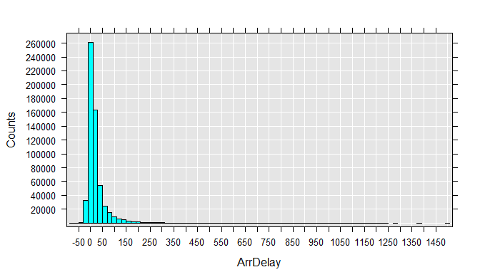
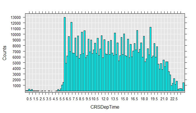
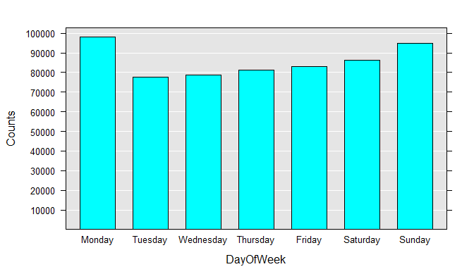
To get a better feel for the data, you can draw histograms for each variable. Run each rxHistogram function one at a time. The histogram is rendered in the R Plot pane.
options("device.ask.default" = T)
rxHistogram(~ArrDelay, data=airXdfData)
rxHistogram(~CRSDepTime, data=airXdfData)
rxHistogram(~DayOfWeek, data=airXdfData)
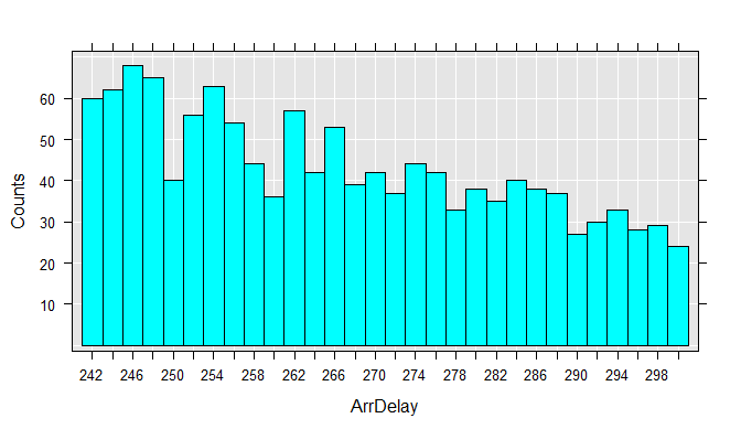
We can also easily extract a subsample of the data file into a data frame in memory. For example, we can look at just the flights that were between 4 and 5 hours late:
myData <- rxDataStep(inData = airXdfData,
rowSelection = ArrDelay > 240 & ArrDelay <= 300,
	varsToKeep = c("ArrDelay", "DayOfWeek"))
rxHistogram(~ArrDelay, data = myData)
Load a data subset
This exercise shows you how to use rxDataStep to read an arbitrary chunk of the dataset into a data frame for further examination. As a first step, lets get the number of rows, columns, and return the initial rows to better understand the available data. Standard R methods provide this information.
nrow(airXdfData)
ncol(airXdfData)
head(airXdfData)

> nrow(airXdfData)
[1] 600000
> ncol(airXdfData)
[1] 3
> head(airXdfData)
	ArrDelay CRSDepTime DayOfWeek
1        6   9.666666    Monday
2       -8  19.916666    Monday
3       -2  13.750000    Monday
4        1  11.750000    Monday
5       -2   6.416667    Monday
6      -14  13.833333    Monday
From nrow we see that the number of rows is 600,000. To read 10 rows into a data frame starting with the 100,000th row:
airXdfDataSmall <- rxDataStep(inData=airXdfData, numRows=10, startRow=100000)
airXdfDataSmall
This code should generate the following output:
	ArrDelay CRSDepTime DayOfWeek
1        -2  11.416667  Saturday
2        39   9.916667    Friday
3        NA  10.033334    Monday
4         1  17.000000    Friday
5       -17   9.983334 Wednesday
6         8  21.250000  Saturday
7        -9   6.250000    Friday
8       -11  15.000000    Friday
9         4  20.916666    Sunday
10       -8   6.500000  Thursday
You can now compute summary statistics on the reduced dataset
Create a new dataset with variable transformations
In this task, use the rxDataStep function to create a new dataset containing the variables in airXdfData plus additional variables created through transformations. Typically additional variables are created using the transforms argument. You can refer to Transform functions for information. Remember that all expressions used in transforms must be able to be processed on a chunk of data at a time.
In the example below, three new variables are created.
- Late is a logical variable set to TRUE (or 1) if the flight was more than 15 minutes late in arriving.
- DepHour is an integer variable indicating the hour of the departure.
- Night is also a logical variable, set to TRUE (or 1) if the flight departed between 10 P.M. and 5 A.M.
The rxDataStep function will read the existing dataset and perform the transformations chunk by chunk, and create a new dataset.
	airExtraDS <- rxDataStep(inData=airXdfData, outFile="c:/users/temp/ADS2.xdf",
		transforms=list(
			Late = ArrDelay > 15,
			DepHour = as.integer(CRSDepTime),
			Night = DepHour >= 20 | DepHour <= 5))

	rxGetInfo(airExtraDS, getVarInfo=TRUE, numRows=5)
You should see the following information in your output:
	C:\Users\TEMP\ADS2.xdf
	Number of observations: 6e+05
	Number of variables: 6
	Number of blocks: 2
	Compression type: zlib
	Variable information:
	Var 1: ArrDelay, Type: integer, Low/High: (-86, 1490)
	Var 2: CRSDepTime, Type: numeric, Storage: float32, Low/High: (0.0167, 23.9833)
	Var 3: DayOfWeek
	       7 factor levels: Monday Tuesday Wednesday Thursday Friday Saturday Sunday
	Var 4: Late, Type: logical, Low/High: (0, 1)
	Var 5: DepHour, Type: integer, Low/High: (0, 23)
	Var 6: Night, Type: logical, Low/High: (0, 1)
	Data (5 rows starting with row 1):
	  ArrDelay CRSDepTime DayOfWeek  Late DepHour Night
	1        6   9.666666    Monday FALSE       9 FALSE
	2       -8  19.916666    Monday FALSE      19 FALSE
	3       -2  13.750000    Monday FALSE      13 FALSE
	4        1  11.750000    Monday FALSE      11 FALSE
	5       -2   6.416667    Monday FALSE       6 FALSE
Next steps
This tutorial demonstrated data import and exploration, but there are several more tutorials covering more scenarios, including instructions for working with bigger datasets.
- Tutorial: Visualize and analyze data
- Analyze large data with RevoScaleR and airline flight delay data
- Example: Analyzing loan data with RevoScaleR
- Example: Analyzing census data with RevoScaleR
Try demo scripts
Another way to learn about RevoScaleR is through demo scripts. Scripts provided in your Machine Learning Server installation contain code that's very similar to what you see in the tutorials.
Demo scripts are located in the demoScripts subdirectory of your Machine Learning Server installation. On Windows, this is typically:
C:\Program Files\Microsoft\R Client\R_SERVER\library\RevoScaleR\demoScripts
Watch this video
This 30-minute video is the second in a 4-part video series. It demonstrates RevoScaleR functions for data ingestion.
Tip
This video shows you how to create a source object for a list of files by using the R list.files function and patterns for selecting specific file names. It uses the multiple mortDefaultSmall.csv files to show the approach. To create an XDF comprised of all the files, use the following syntax: mySourceFiles <- list.files(rxGetOption("sampleDataDir"), pattern = "mortDefaultSmall\\d</em>.csv", full.names=TRUE).
Overcome R Client data chunking limitations by pushing compute context or migrating to Machine Learning Server
Data chunking is a RevoScaleR capability that partitions data into multiple parts for processing in parallel, reassembling it later for analysis. It's one of the key mechanisms by which RevoScaleR processes and analyzes very large datasets.
In Machine Learning Server, chunking functionality is available only when RevoScaleR functions are executed on Machine Learning Server for Windows, Teradata, SQL Server, Linux, or Hadoop. You cannot use chunking on systems that have just Microsoft R Client. R Client requires that data fits into available memory. Moreover, it can only use a maximum of two threads for analysis. Internally, when RevoScaleR is running in R Client, the blocksPerRead argument is deliberately, which results in all data being read into memory.
You can work around this limitation by writing script on R Client, but then pushing the compute context from R Client to a remote Machine Learning Server instance. Optionally, you could use Machine Learning Server. Developers can install the developer edition of Machine Learning Server which is a full-featured Machine Learning Server, but licensed for development workstations instead of production servers. For more information, see Machine Learning Server.
See Also
Machine Learning Server
Getting Started with Hadoop and RevoScaleR
Parallel and distributed computing in Machine Learning Server
Importing data
ODBC data import
RevoScaleR Functions