Many-to-many relationship guidance
This article targets you as a data modeler working with Power BI Desktop. It describes three different many-to-many modeling scenarios. It also provides you with guidance on how to successfully design for them in your models.
Note
An introduction to model relationships is not covered in this article. If you're not completely familiar with relationships, their properties or how to configure them, we recommend that you first read the Model relationships in Power BI Desktop article.
It's also important that you have an understanding of star schema design. For more information, see Understand star schema and the importance for Power BI.
There are, in fact, three many-to-many scenarios. They can occur when you're required to:
- Relate two dimension-type tables
- Relate two fact-type tables
- Relate higher grain fact-type tables, when the fact-type table stores rows at a higher grain than the dimension-type table rows
Note
Power BI now natively supports many-to-many relationships. For more information, see Apply many-many relationships in Power BI Desktop.
Relate many-to-many dimensions
Let's consider the first many-to-many scenario type with an example. The classic scenario relates two entities: bank customers and bank accounts. Consider that customers can have multiple accounts, and accounts can have multiple customers. When an account has multiple customers, they're commonly called joint account holders.
Modeling these entities is straight forward. One dimension-type table stores accounts, and another dimension-type table stores customers. As is characteristic of dimension-type tables, there's an ID column in each table. To model the relationship between the two tables, a third table is required. This table is commonly referred to as a bridging table. In this example, it's purpose is to store one row for each customer-account association. Interestingly, when this table only contains ID columns, it's called a factless fact table.
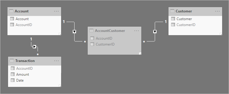
Here's a simplistic model diagram of the three tables.

The first table is named Account, and it contains two columns: AccountID and Account. The second table is named AccountCustomer, and it contains two columns: AccountID and CustomerID. The third table is named Customer, and it contains two columns: CustomerID and Customer. Relationships don't exist between any of the tables.
Two one-to-many relationships are added to relate the tables. Here's an updated model diagram of the related tables. A fact-type table named Transaction has been added. It records account transactions. The bridging table and all ID columns have been hidden.
To help describe how the relationship filter propagation works, the model diagram has been modified to reveal the table rows.
Note
It's not possible to display table rows in the Power BI Desktop model diagram. It's done in this article to support the discussion with clear examples.
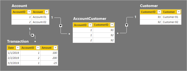
The row details for the four tables are described in the following bulleted list:
- The Account table has two rows:
- AccountID 1 is for Account-01
- AccountID 2 is for Account-02
- The Customer table has two rows:
- CustomerID 91 is for Customer-91
- CustomerID 92 is for Customer-92
- The AccountCustomer table has three rows:
- AccountID 1 is associated with CustomerID 91
- AccountID 1 is associated with CustomerID 92
- AccountID 2 is associated with CustomerID 92
- The Transaction table has three rows:
- Date January 1 2019, AccountID 1, Amount 100
- Date February 2 2019, AccountID 2, Amount 200
- Date March 3 2019, AccountID 1, Amount -25
Let's see what happens when the model is queried.
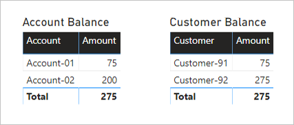
Below are two visuals that summarize the Amount column from the Transaction table. The first visual groups by account, and so the sum of the Amount columns represents the account balance. The second visual groups by customer, and so the sum of the Amount columns represents the customer balance.
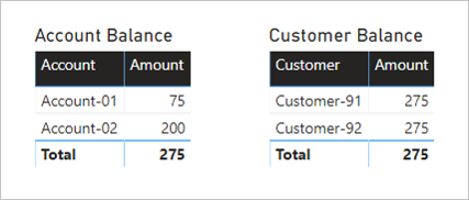
The first visual is titled Account Balance, and it has two columns: Account and Amount. It displays the following result:
- Account-01 balance amount is 75
- Account-02 balance amount is 200
- The total is 275
The second visual is titled Customer Balance, and it has two columns: Customer and Amount. It displays the following result:
- Customer-91 balance amount is 275
- Customer-92 balance amount is 275
- The total is 275
A quick glance at the table rows and the Account Balance visual reveals that the result is correct, for each account and the total amount. It's because each account grouping results in a filter propagation to the Transaction table for that account.
However, something doesn't appear correct with the Customer Balance visual. Each customer in the Customer Balance visual has the same balance as the total balance. This result could only be correct if every customer was a joint account holder of every account. That's not the case in this example. The issue is related to filter propagation. It's not flowing all the way to the Transaction table.
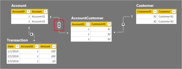
Follow the relationship filter directions from the Customer table to the Transaction table. It should be apparent that the relationship between the Account and AccountCustomer table is propagating in the wrong direction. The filter direction for this relationship must be set to Both.
As expected, there has been no change to the Account Balance visual.
The Customer Balance visuals, however, now displays the following result:
- Customer-91 balance amount is 75
- Customer-92 balance amount is 275
- The total is 275
The Customer Balance visual now displays a correct result. Follow the filter directions for yourself, and see how the customer balances were calculated. Also, understand that the visual total means all customers.
Someone unfamiliar with the model relationships could conclude that the result is incorrect. They might ask: Why isn't the total balance for Customer-91 and Customer-92 equal to 350 (75 + 275)?
The answer to their question lies in understanding the many-to-many relationship. Each customer balance can represent the addition of multiple account balances, and so the customer balances are non-additive.
Relate many-to-many dimensions guidance
When you have a many-to-many relationship between dimension-type tables, we provide the following guidance:
- Add each many-to-many related entity as a model table, ensuring it has a unique identifier (ID) column
- Add a bridging table to store associated entities
- Create one-to-many relationships between the three tables
- Configure one bi-directional relationship to allow filter propagation to continue to the fact-type tables
- When it isn't appropriate to have missing ID values, set the Is Nullable property of ID columns to FALSE—data refresh will then fail if missing values are sourced
- Hide the bridging table (unless it contains additional columns or measures required for reporting)
- Hide any ID columns that aren't suitable for reporting (for example, when IDs are surrogate keys)
- If it makes sense to leave an ID column visible, ensure that it's on the "one" slide of the relationship—always hide the "many" side column. It results in the best filter performance.
- To avoid confusion or misinterpretation, communicate explanations to your report users—you can add descriptions with text boxes or visual header tooltips
We don't recommend you relate many-to-many dimension-type tables directly. This design approach requires configuring a relationship with a many-to-many cardinality. Conceptually it can be achieved, yet it implies that the related columns will contain duplicate values. It's a well-accepted design practice, however, that dimension-type tables have an ID column. Dimension-type tables should always use the ID column as the "one" side of a relationship.
Relate many-to-many facts
The second many-to-many scenario type involves relating two fact-type tables. Two fact-type tables can be related directly. This design technique can be useful for quick and simple data exploration. However, and to be clear, we generally don't recommend this design approach. We'll explain why later in this section.
Let's consider an example that involves two fact-type tables: Order and Fulfillment. The Order table contains one row per order line, and the Fulfillment table can contains zero or more rows per order line. Rows in the Order table represent sales orders. Rows in the Fulfillment table represent order items that have been shipped. A many-to-many relationship relates the two OrderID columns, with filter propagation only from the Order table (Order filters Fulfillment).
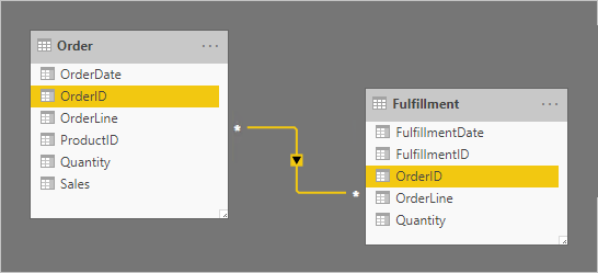
The relationship cardinality is set to many-to-many to support storing duplicate OrderID values in both tables. In the Order table, duplicate OrderID values can exist because an order can have multiple lines. In the Fulfillment table, duplicate OrderID values can exist because orders may have multiple lines, and order lines can be fulfilled by many shipments.
Let's now take a look at the table rows. In the Fulfillment table, notice that order lines can be fulfilled by multiple shipments. (The absence of an order line means the order is yet to be fulfilled.)
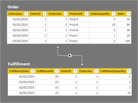
The row details for the two tables are described in the following bulleted list:
- The Order table has five rows:
- OrderDate January 1 2019, OrderID 1, OrderLine 1, ProductID Prod-A, OrderQuantity 5, Sales 50
- OrderDate January 1 2019, OrderID 1, OrderLine 2, ProductID Prod-B, OrderQuantity 10, Sales 80
- OrderDate February 2 2019, OrderID 2, OrderLine 1, ProductID Prod-B, OrderQuantity 5, Sales 40
- OrderDate February 2 2019, OrderID 2, OrderLine 2, ProductID Prod-C, OrderQuantity 1, Sales 20
- OrderDate March 3 2019, OrderID 3, OrderLine 1, ProductID Prod-C, OrderQuantity 5, Sales 100
- The Fulfillment table has four rows:
- FulfillmentDate January 1 2019, FulfillmentID 50, OrderID 1, OrderLine 1, FulfillmentQuantity 2
- FulfillmentDate February 2 2019, FulfillmentID 51, OrderID 2, OrderLine 1, FulfillmentQuantity 5
- FulfillmentDate February 2 2019, FulfillmentID 52, OrderID 1, OrderLine 1, FulfillmentQuantity 3
- FulfillmentDate January 1 2019, FulfillmentID 53, OrderID 1, OrderLine 2, FulfillmentQuantity 10
Let's see what happens when the model is queried. Here's a table visual comparing order and fulfillment quantities by the Order table OrderID column.
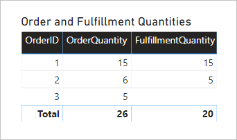
The visual presents an accurate result. However, the usefulness of the model is limited—you can only filter or group by the Order table OrderID column.
Relate many-to-many facts guidance
Generally, we don't recommend relating two fact-type tables directly using many-to-many cardinality. The main reason is because the model won't provide flexibility in the ways you report visuals filter or group. In the example, it's only possible for visuals to filter or group by the Order table OrderID column. An additional reason relates to the quality of your data. If your data has integrity issues, it's possible some rows may be omitted during querying due to the nature of the limited relationship. For more information, see Model relationships in Power BI Desktop (Relationship evaluation).
Instead of relating fact-type tables directly, we recommend you adopt Star Schema design principles. You do it by adding dimension-type tables. The dimension-type tables then relate to the fact-type tables by using one-to-many relationships. This design approach is robust as it delivers flexible reporting options. It lets you filter or group using any of the dimension-type columns, and summarize any related fact-type table.
Let's consider a better solution.
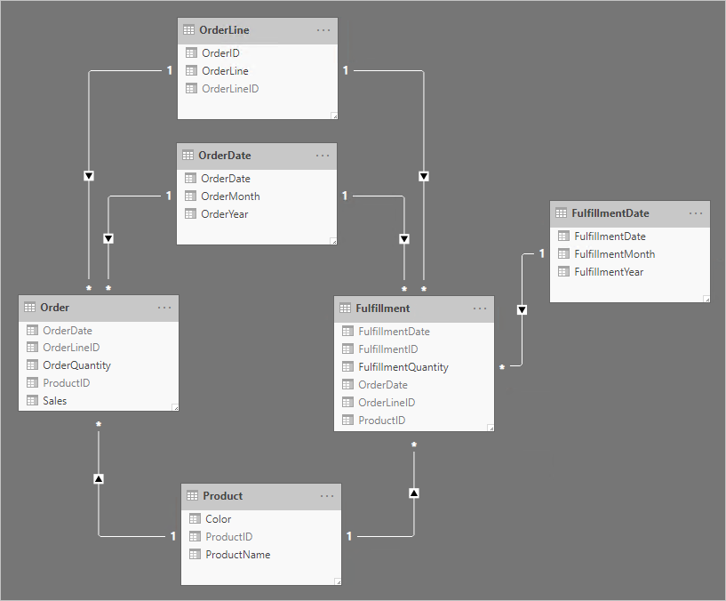
Notice the following design changes:
- The model now has four additional tables: OrderLine, OrderDate, Product, and FulfillmentDate
- The four additional tables are all dimension-type tables, and one-to-many relationships relate these tables to the fact-type tables
- The OrderLine table contains an OrderLineID column, which represents the OrderID value multiplied by 100, plus the OrderLine value—a unique identifier for each order line
- The Order and Fulfillment tables now contain an OrderLineID column, and they no longer contain the OrderID and OrderLine columns
- The Fulfillment table now contains OrderDate and ProductID columns
- The FulfillmentDate table relates only to the Fulfillment table
- All unique identifier columns are hidden
Taking the time to apply star schema design principles delivers the following benefits:
- Your report visuals can filter or group by any visible column from the dimension-type tables
- Your report visuals can summarize any visible column from the fact-type tables
- Filters applied to the OrderLine, OrderDate, or Product tables will propagate to both fact-type tables
- All relationships are one-to-many, and each relationship is a regular relationship. Data integrity issues won't be masked. For more information, see Model relationships in Power BI Desktop (Relationship evaluation).
Relate higher grain facts
This many-to-many scenario is very different from the other two already described in this article.
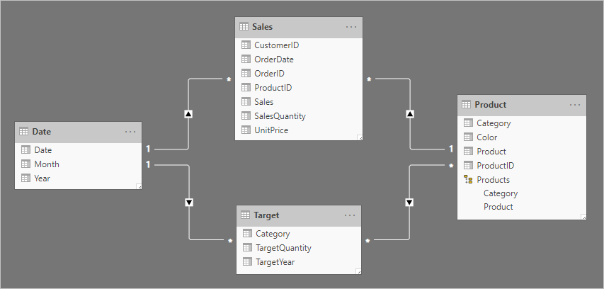
Let's consider an example involving four tables: Date, Sales, Product, and Target. The Date and Product are dimension-type tables, and one-to-many relationships relate each to the Sales fact-type table. So far, it represents a good star schema design. The Target table, however, is yet to be related to the other tables.
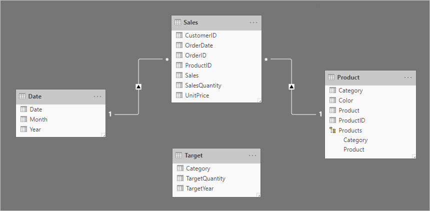
The Target table contains three columns: Category, TargetQuantity, and TargetYear. The table rows reveal a granularity of year and product category. In other words, targets—used to measure sales performance—are set each year for each product category.
Because the Target table stores data at a higher level than the dimension-type tables, a one-to-many relationship cannot be created. Well, it's true for just one of the relationships. Let's explore how the Target table can be related to the dimension-type tables.
Relate higher grain time periods
A relationship between the Date and Target tables should be a one-to-many relationship. It's because the TargetYear column values are dates. In this example, each TargetYear column value is the first date of the target year.
Tip
When storing facts at a higher time granularity than day, set the column data type to Date (or Whole number if you're using date keys). In the column, store a value representing the first day of the time period. For example, a year period is recorded as January 1 of the year, and a month period is recorded as the first day of that month.
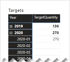
Care must be taken, however, to ensure that month or date level filters produce a meaningful result. Without any special calculation logic, report visuals may report that target dates are literally the first day of each year. All other days—and all months except January—will summarize the target quantity as BLANK.
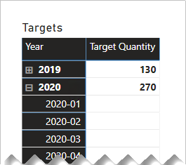
The following matrix visual shows what happens when the report user drills from a year into its months. The visual is summarizing the TargetQuantity column. (The Show items with no data option has been enabled for the matrix rows.)
To avoid this behavior, we recommend you control the summarization of your fact data by using measures. One way to control the summarization is to return BLANK when lower-level time periods are queried. Another way—defined with some sophisticated DAX—is to apportion values across lower-level time periods.
Consider the following measure definition that uses the ISFILTERED DAX function. It only returns a value when the Date or Month columns aren't filtered.
Target Quantity =
IF(
    NOT ISFILTERED('Date'[Date])
        && NOT ISFILTERED('Date'[Month]),
    SUM(Target[TargetQuantity])
)
The following matrix visual now uses the Target Quantity measure. It shows that all monthly target quantities are BLANK.
Relate higher grain (non-date)
A different design approach is required when relating a non-date column from a dimension-type table to a fact-type table (and it's at a higher grain than the dimension-type table).
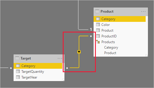
The Category columns (from both the Product and Target tables) contains duplicate values. So, there's no "one" for a one-to-many relationship. In this case, you'll need to create a many-to-many relationship. The relationship should propagate filters in a single direction, from the dimension-type table to the fact-type table.
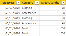
Let's now take a look at the table rows.
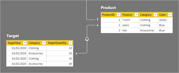
In the Target table, there are four rows: two rows for each target year (2019 and 2020), and two categories (Clothing and Accessories). In the Product table, there are three products. Two belong to the clothing category, and one belongs to the accessories category. One of the clothing colors is green, and the remaining two are blue.
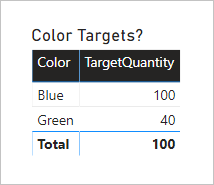
A table visual grouping by the Category column from the Product table produces the following result.
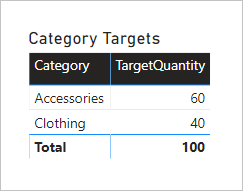
This visual produces the correct result. Let's now consider what happens when the Color column from the Product table is used to group target quantity.
The visual produces a misrepresentation of the data. What is happening here?
A filter on the Color column from the Product table results in two rows. One of the rows is for the Clothing category, and the other is for the Accessories category. These two category values are propagated as filters to the Target table. In other words, because the color blue is used by products from two categories, those categories are used to filter the targets.
To avoid this behavior, as described earlier, we recommend you control the summarization of your fact data by using measures.
Consider the following measure definition. Notice that all Product table columns that are beneath the category level are tested for filters.
Target Quantity =
IF(
    NOT ISFILTERED('Product'[ProductID])
        && NOT ISFILTERED('Product'[Product])
        && NOT ISFILTERED('Product'[Color]),
    SUM(Target[TargetQuantity])
)
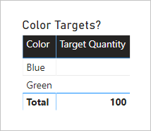
The following table visual now uses the Target Quantity measure. It shows that all color target quantities are BLANK.
The final model design looks like the following.
Relate higher grain facts guidance
When you need to relate a dimension-type table to a fact-type table, and the fact-type table stores rows at a higher grain than the dimension-type table rows, we provide the following guidance:
- For higher grain fact dates:
- In the fact-type table, store the first date of the time period
- Create a one-to-many relationship between the date table and the fact-type table
- For other higher grain facts:
- Create a many-to-many relationship between the dimension-type table and the fact-type table
- For both types:
- Control summarization with measure logic—return BLANK when lower-level dimension-type columns are used to filter or group
- Hide summarizable fact-type table columns—this way, only measures can be used to summarize the fact-type table
Related content
For more information related to this article, check out the following resources:
Feedback
Coming soon: Throughout 2024 we will be phasing out GitHub Issues as the feedback mechanism for content and replacing it with a new feedback system. For more information see: https://aka.ms/ContentUserFeedback.
Submit and view feedback for