Tutorial: Create a predictive model in R with SQL machine learning
Applies to: ![]() SQL Server 2016 (13.x) and later
SQL Server 2016 (13.x) and later ![]() Azure SQL Managed Instance
Azure SQL Managed Instance
In part three of this four-part tutorial series, you'll train a predictive model in R. In the next part of this series, you'll deploy this model in a SQL Server database with Machine Learning Services or on Big Data Clusters.
In part three of this four-part tutorial series, you'll train a predictive model in R. In the next part of this series, you'll deploy this model in a SQL Server database with Machine Learning Services.
In part three of this four-part tutorial series, you'll train a predictive model in R. In the next part of this series, you'll deploy this model in a database with SQL Server R Services.
In part three of this four-part tutorial series, you'll train a predictive model in R. In the next part of this series, you'll deploy this model in an Azure SQL Managed Instance database with Machine Learning Services.
In this article, you'll learn how to:
- Train two machine learning models
- Make predictions from both models
- Compare the results to choose the most accurate model
In part one, you learned how to restore the sample database.
In part two, you learned how to load the data from a database into a Python data frame and prepare the data in R.
In part four, you'll learn how to store the model in a database, and then create stored procedures from the Python scripts you developed in parts two and three. The stored procedures will run in on the server to make predictions based on new data.
Prerequisites
Part three of this tutorial series assumes you have fulfilled the prerequisites of part one, and completed the steps in part two.
Train two models
To find the best model for the ski rental data, create two different models (linear regression and decision tree) and see which one is predicting more accurately. You'll use the data frame rentaldata that you created in part one of this series.
#First, split the dataset into two different sets:
# one for training the model and the other for validating it
train_data = rentaldata[rentaldata$Year < 2015,];
test_data  = rentaldata[rentaldata$Year == 2015,];


#Use the RentalCount column to check the quality of the prediction against actual values
actual_counts <- test_data$RentalCount;

#Model 1: Use lm to create a linear regression model, trained with the training data set
model_lm <- lm(RentalCount ~  Month + Day + WeekDay + Snow + Holiday, data = train_data);

#Model 2: Use rpart to create a decision tree model, trained with the training data set
library(rpart);
model_rpart  <- rpart(RentalCount ~ Month + Day + WeekDay + Snow + Holiday, data = train_data);
Make predictions from both models
Use a predict function to predict the rental counts using each trained model.
#Use both models to make predictions using the test data set.
predict_lm <- predict(model_lm, test_data)
predict_lm <- data.frame(RentalCount_Pred = predict_lm, RentalCount = test_data$RentalCount,
                         Year = test_data$Year, Month = test_data$Month,
                         Day = test_data$Day, Weekday = test_data$WeekDay,
                         Snow = test_data$Snow, Holiday = test_data$Holiday)

predict_rpart  <- predict(model_rpart,  test_data)
predict_rpart <- data.frame(RentalCount_Pred = predict_rpart, RentalCount = test_data$RentalCount,
                         Year = test_data$Year, Month = test_data$Month,
                         Day = test_data$Day, Weekday = test_data$WeekDay,
                         Snow = test_data$Snow, Holiday = test_data$Holiday)

#To verify it worked, look at the top rows of the two prediction data sets.
head(predict_lm);
head(predict_rpart);
    RentalCount_Pred  RentalCount  Month  Day  WeekDay  Snow  Holiday
1         27.45858          42       2     11     4      0       0
2        387.29344         360       3     29     1      0       0
3         16.37349          20       4     22     4      0       0
4         31.07058          42       3      6     6      0       0
5        463.97263         405       2     28     7      1       0
6        102.21695          38       1     12     2      1       0
    RentalCount_Pred  RentalCount  Month  Day  WeekDay  Snow  Holiday
1          40.0000          42       2     11     4      0       0
2         332.5714         360       3     29     1      0       0
3          27.7500          20       4     22     4      0       0
4          34.2500          42       3      6     6      0       0
5         645.7059         405       2     28     7      1       0
6          40.0000          38       1     12     2      1       0
Compare the results
Now you want to see which of the models gives the best predictions. A quick and easy way to do this is to use a basic plotting function to view the difference between the actual values in your training data and the predicted values.
#Use the plotting functionality in R to visualize the results from the predictions
par(mfrow = c(1, 1));
plot(predict_lm$RentalCount_Pred - predict_lm$RentalCount, main = "Difference between actual and predicted. lm")
plot(predict_rpart$RentalCount_Pred  - predict_rpart$RentalCount,  main = "Difference between actual and predicted. rpart")
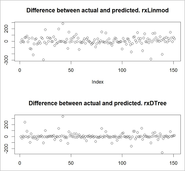
It looks like the decision tree model is the more accurate of the two models.
Clean up resources
If you're not going to continue with this tutorial, delete the TutorialDB database.
Next steps
In part three of this tutorial series, you learned how to:
- Train two machine learning models
- Make predictions from both models
- Compare the results to choose the most accurate model
To deploy the machine learning model you've created, follow part four of this tutorial series:
Feedback
Coming soon: Throughout 2024 we will be phasing out GitHub Issues as the feedback mechanism for content and replacing it with a new feedback system. For more information see: https://aka.ms/ContentUserFeedback.
Submit and view feedback for