Use IPython in the Interactive window
Applies to: ![]() Visual Studio
Visual Studio ![]() Visual Studio for Mac
Visual Studio for Mac
Note
This article applies to Visual Studio 2017. If you're looking for the latest Visual Studio documentation, see Visual Studio documentation. We recommend upgrading to the latest version of Visual Studio. Download it here
The Visual Studio Interactive window in IPython mode is an advanced yet user-friendly interactive development environment that has Interactive Parallel Computing features. This article walks through using IPython in the Visual Studio Interactive window, in which all of the regular Interactive window features are also available.
For this walkthrough, you will need to have installed IPython, numpy and matplotlib. If you are using Anaconda, these libraries are already installed. The rest of the walkthrough assumes you are using Anaconda.
Note
IronPython does not support IPython, despite the fact that you can select it on the Interactive Options form. For more information see the feature request.
Open Visual Studio, switch to the Python Environments window (View > Other Windows > Python Environments), and select an Anaconda environment.
Examine the Packages (Conda) tab (which may appear as pip or Packages) for that environment to make sure that
ipythonandmatplotlibare listed. If not, install them here. (See Python Environments windows - Packages tab.)Select the Overview tab and select Use IPython interactive mode. (In Visual Studio 2015, select Configure interactive options to open the Options dialog, then set Interactive Mode to IPython, and select OK).
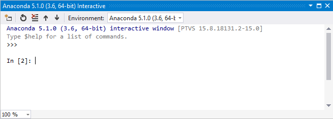
Select Open interactive window to bring up the Interactive window in IPython mode. You may need to reset the window if you have just changed the interactive mode; you might also need to press Enter if only a >>> prompt appears, so that you get a prompt like In [2].
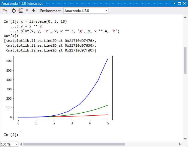
Enter the following code:
import matplotlib.pyplot as plt
import numpy as np

x = np.linspace(0, 5, 10)
y = x ** 2
plt.plot(x, y, 'r', x, x ** 3, 'g', x, x ** 4, 'b')
After entering the last line, you should see an inline graph (which you can resize by dragging on the lower right-hand corner if desired).
Instead of typing in the REPL, you can instead write code in the editor, select it, right-click, and select the Send to Interactive command (or press Ctrl+Enter). Try pasting the code below into a new file in the editor, selecting it with Ctrl+A, then sending to the Interactive window. (Visual Studio sends the code as one unit to avoid giving you intermediate or partial graphs. And if you don't have a Python project open with a different environment selected, Visual Studio opens an Interactive window for whatever environment is selected as your default in the Python Environments window.)
from mpl_toolkits.mplot3d import Axes3D
import matplotlib.pyplot as plt
import numpy as np
fig = plt.figure()
ax = fig.add_subplot(111, projection='3d')
for c, z in zip(['r', 'g', 'b', 'y'], [30, 20, 10, 0]):
    xs = np.arange(20)
    ys = np.random.rand(20)
    # You can provide either a single color or an array. To demonstrate this,
    # the first bar of each set is colored cyan.
    cs = [c] * len(xs)
    cs[0] = 'c'
    ax.bar(xs, ys, zs=z, zdir='y', color=cs, alpha=0.8)

ax.set_xlabel('X')
ax.set_ylabel('Y')
ax.set_zlabel('Z')
plt.show()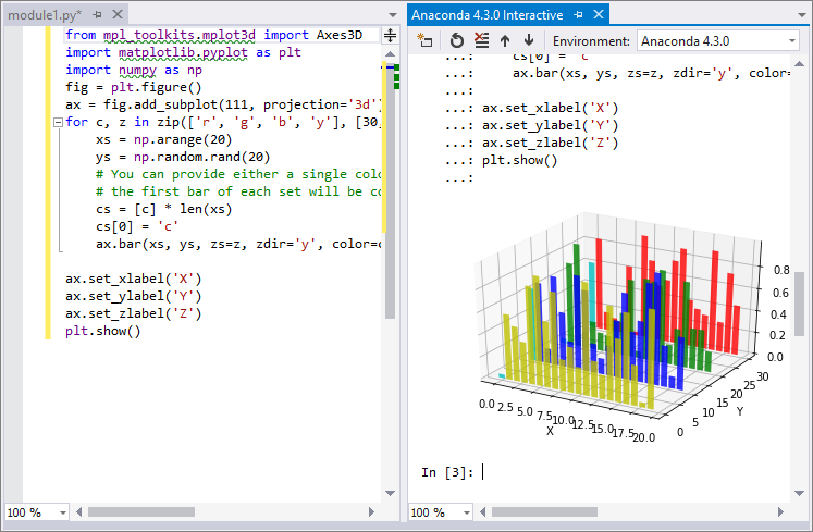
To see the graphs outside of the Interactive window, run the code instead using the Debug > Start without Debugging command.
IPython has many other useful features such as escaping to the system shell, variable substitution, capturing output, etc. Refer to the IPython documentation for more.
See also
- The Azure Data Science Virtual Machine is pre-configured to run Jupyter notebooks along with a wide range of other data science tools.