How to summarize data using RevoScaleR
Important
This content is being retired and may not be updated in the future. The support for Machine Learning Server will end on July 1, 2022. For more information, see What's happening to Machine Learning Server?
Summary statistics can help you understand the characteristics and shape of an unfamiliar data set. In RevoScaleR, you can use the rxGetVarInfo function to learn more about variables in the data set, and rxSummary for statistical measures. The rxSummary function also provides a count of observations, and the number of missing values (if any).
This article teaches by example, using built-in sample data sets so that you can practice each skill. It covers the following tasks:
- List variable metadata including name, description, type, labels, Low/High values
- Compute summary statistics: mean, standard deviation, minimum, maximum values
- Compute summary statistics for factor variables
- Create temporary factor variables used in computations
- Compute summary statistics on a row subset
- Execute in-flight data transformations
- Compute and plot a Lorenz curve
- Tips for wide data sets
List variable information
The rxGetVarInfo function returns information about the variables in a data frame or .xdf file, including variable names, descriptions, type, and high and low values. The following examples, based on the built-in sample Census data set, demonstrate function usage.
# Load data, store variable metadata as censusWorkerInfo, and return variable names.

readPath <- rxGetOption("sampleDataDir")
censusWorkers <- file.path(readPath, "CensusWorkers.xdf")
censusWorkerInfo <- rxGetVarInfo(censusWorkers)
names(censusWorkerInfo)
The names function is a base R function, which is called on the object to return the following variable names:
[1] "age" "incwage" "perwt" "sex" "wkswork1" "state"
Once you have a variable name, you can drill down further to examine its metadata. This is the output for age:
names(censusWorkerInfo$age)

	[1] "description" "varType" "storage" "low" "high"
Numeric variables include Low/High values. The Low/High values do not necessarily indicate the minimum and maximum of a numeric or integer variable. Rather, they indicate the values RevoScaleR uses to establish the lowest and highest factor levels when treating the variable as a factor. For practical purposes, this is more helpful for data visualization than a true minimum or maximum on the variable. For example, suppose you want to create histograms or hexbin plots, treating the numerical data as categorical, with levels corresponding to the plotting bins. In this scenario, it is often convenient to cut off the highest and lowest data points, and the Low/High values provide this information.
This example demonstrates getting the High value from the age variable:
censusWorkerInfo$age$high

	[1] 65
Similarly, the Low value is obtained as follows:
censusWorkerInfo$age$low

	[1] 20
Suppose you are interested in workers between the ages of 30 and 50. You could create a copy of the data file in the working directory, set the High/Low fields as follows and then treat age as a factor in subsequent analysis:
outputDir <- rxGetOption("outDataPath")
tempCensusWorkers <- file.path(outputDir, "tempCensusWorkers.xdf")
file.copy(from = censusWorkers, to = tempCensusWorkers)
censusWorkerInfo$age$low <- 35
censusWorkerInfo$age$high <- 50
rxSetVarInfo(censusWorkerInfo, tempCensusWorkers)
rxSummary(~F(age), data = tempCensusWorkers)
Results (restricted to the 35 to 50 age range):
Call:
rxSummary(formula = ~F(age), data = tempCensusWorkers)

Summary Statistics Results for: ~F(age)
File name:
	C:\YourOutDir\tempCensusWorkers.xdf
Number of valid observations: 351121

Category Counts for F_age
Number of categories: 16
Number of valid observations: 158309
Number of missing observations: 192812

	F_age Counts
	35     9743
	36     9888
	37     9860
	38    10211
	39    10378
	40    10756
	41    10503
	42    10511
	43    10296
	44    10122
	45    10074
	46     9703
	47     9527
	48     9093
	49     8776
	50     8868
To reset the low and high values, repeat the previous steps with the original values:
censusWorkerInfo$age$low <- 20
censusWorkerInfo$age$high <- 65
rxSetVarInfo(censusWorkerInfo, "tempCensusWorkers.xdf")
Compute summary statistics
The rxSummary function provides descriptive statistics using a formula argument similar to that used in R’s modeling functions. The formula specifies the independent variables to summarize.
The basic structure of a formula is a tilde symbol "~" with one or more independent or right-hand variables, separated by "+". To include all of the variables, you can append a dot (.) to the tilde as "~.".
The rxSummary function also takes a data object as the source of the variables.
For example, returning to the CensusWorkers sample, run the following script to obtain a data summary of that file:
# Formulas in rxSummary

readPath <- rxGetOption("sampleDataDir")
censusWorkers <- file.path(readPath, "CensusWorkers.xdf")
rxSummary(~ age + incwage + perwt + sex + wkswork1, data = censusWorkers)
For each term in the formula, the mean, standard deviation, minimum, maximum, and number of valid observations is shown. If rxSummary includes byTerm=FALSE, the observations (rows) containing missing values for any of the specified variables are omitted in calculating the summary. Cell counts for categorical variables are included.
Results
Call:
rxSummary(formula = ~age + incwage + perwt + sex + wkswork1,
	data = censusWorkers)

Summary Statistics Results for: ~age + incwage + perwt + sex + wkswork1
Data: censusWorkers (RxXdfData Data Source)
File name: C:/Program Files/Microsoft/ML Server/R_SERVER/library/RevoScaleR/SampleData/CensusWorkers.xdf
Number of valid observations: 351121

	Name     Mean        StdDev       Min Max    ValidObs MissingObs
	age         40.42814    11.385017 20      65 351121   0
	incwage  35333.83894 40444.544084  0  354000 351121   0
	perwt       20.34423     9.633100  2     168 351121   0
	wkswork1    48.62566     6.953843 21      52 351121   0

Category Counts for sex
Number of categories: 2
Number of valid observations: 351121
Number of missing observations: 0

	sex    Counts
	Male   189344
	Female 161777
Compute median values
You might have noticed that rxSummary does not compute a median value for each variable. This is because rxSummary only produces statistics that can be computed in chunks, and a median computation is not a chunkable calculation. Median calculations are predicated on a sort operation, which is expensive on large data sets, and thus excluded from rxSummary.
Assuming your data set fits in memory, you could get the median value of a given variable using the base R median function:
# Load data into a dataframe
mydataframe <- rxImport(censusWorkers)

# As verification, print values of a numeric variable, such as age
mydataframe$age

# Compute the median age
median(mydataframe$age)
Results
[1] 40
For larger disk-bound datasets, you should use visualization techniques to uncover skewness in the underlying data.
Compute summary statistics on factor variables
You can obtain summary statistics on numeric data that are specific to levels within a variable, such as days of the week, months in a year, age or income levels constructed from column values, and so forth.
To do this, specify an interaction between a numeric variable and a factor variable. For example, using the sample data set AirlineDemoSmall.xdf, use the following command to request a summary of arrival delay by day of week:
rxSummary(~ ArrDelay:DayOfWeek, data = file.path(readPath, "AirlineDemoSmall.xdf"))
Results
The request produces summary statistics for a factor variable, with output for each level.
Call:
rxSummary(formula = ~ArrDelay:DayOfWeek, data = file.path(readPath,
	"AirlineDemoSmall.xdf"))

Summary Statistics Results for: ~ArrDelay:DayOfWeek
Data: file.path(readPath, "AirlineDemoSmall.xdf") (RxXdfData Data Source)
File name: C:/Program Files/Microsoft/ML Server/R_SERVER/library/RevoScaleR/SampleData/AirlineDemoSmall.xdf
Number of valid observations: 6e+05

	Name               Mean     StdDev   Min Max  ValidObs MissingObs
	ArrDelay:DayOfWeek 11.31794 40.68854 -86 1490 582628   17372

Statistics by category (7 categories):

	Category                      DayOfWeek   Means    StdDev   Min Max  ValidObs
	ArrDelay for DayOfWeek=Monday    Monday    12.025604 40.02463 -76 1017 95298
	ArrDelay for DayOfWeek=Tuesday   Tuesday   11.293808 43.66269 -70 1143 74011
	ArrDelay for DayOfWeek=Wednesday Wednesday 10.156539 39.58803 -81 1166 76786
	ArrDelay for DayOfWeek=Thursday  Thursday   8.658007 36.74724 -58 1053 79145
	ArrDelay for DayOfWeek=Friday    Friday    14.804335 41.79260 -78 1490 80142
	ArrDelay for DayOfWeek=Saturday  Saturday  11.875326 45.24540 -73 1370 83851
	ArrDelay for DayOfWeek=Sunday    Sunday    10.331806 37.33348 -86 1202 93395
Note
Interactions provide the one exception to the “responseless” formula mentioned preceding. If you want to obtain the interaction of a continuous variable with one or more factors, you can use a formula of the form y ~ x:z, where y is the continuous variable and x and z are factors. This has precisely the same effect as specifying the formula as ~y:x:z, but is more suggestive of the result: specifically, summary statistics for y at every combination of levels of x and z.
Create a temporary factor variable
You can force RevoScaleR to treat a variable as a factor (with a level for each integer value from the low to high value) by wrapping it with the function call syntax F(). Returning to the CensusWorkers.xdf file, in the following example a factor level is temporarily created for each age from 20 through 65:
rxSummary(~ incwage:F(age), data = censusWorkers)
Results
The results provide not only summary statistics for wage income in the overall data set, but summary statistics on wage income for each age:
Call:
rxSummary(formula = ~incwage:F(age), data = censusWorkers)

Summary Statistics Results for: ~incwage:F(age)
Data: censusWorkers (RxXdfData Data Source)
File name: C:/Program Files/Microsoft/ML Server/R_SERVER/library/RevoScaleR/SampleData/CensusWorkers.xdf
Number of valid observations: 351121

	Name           Mean     StdDev   Min Max    ValidObs MissingObs
	incwage:F(age) 35333.84 40444.54 0   354000 351121   0

Statistics by category (46 categories):

	Category              F_age Means    StdDev   Min Max    ValidObs
	incwage for F(age)=20 20    12669.94 12396.99 0   336000  6500
	incwage for F(age)=21 21    14114.23 12107.81 0   336000  6479
	incwage for F(age)=22 22    15982.00 12374.14 0   336000  6676
	incwage for F(age)=23 23    18503.92 15093.53 0   336000  6884
	incwage for F(age)=24 24    20672.06 14315.67 0   354000  6931
	incwage for F(age)=25 25    23856.25 17319.42 0   336000  7273
	incwage for F(age)=26 26    25938.17 20707.39 0   354000  7116
	incwage for F(age)=27 27    26902.97 20608.09 0   354000  7584
	incwage for F(age)=28 28    28531.59 24185.48 0   354000  8184
	incwage for F(age)=29 29    30153.10 25715.94 0   354000  8889
	incwage for F(age)=30 30    30691.10 26955.27 0   354000  9055
	. . .
If you include an interaction between two factors, the summary provides cell counts for all combinations of levels of the factors. Since the census data has probability weights, you can use the pweights argument to get weighted counts:
rxSummary(~ sex:state, pweights = "perwt", data = censusWorkers)
Results
Call:
rxSummary(formula = ~sex:state, data = censusWorkers, pweights = "perwt")

Summary Statistics Results for: ~sex:state
Data: censusWorkers (RxXdfData Data Source)
File name: C:/Program Files/Microsoft/ML Server/R_SERVER/library/RevoScaleR/SampleData/CensusWorkers.xdf
Probability weights: perwt
Number of valid observations: 351121

Category Counts for sex
Number of categories: 6

	sex    state       Counts
	Male   Connecticut  843736
	Female Connecticut  755843
	Male   Indiana     1517966
	Female Indiana     1289412
	Male   Washington  1504840
	Female Washington  1231489
Compute summary statistics on a row subset
The following example shows how to restrict the analysis to specific rows (in this case, people aged 30 to 39). You can use the low and high arguments of the F() function to restrict the creation of on-the-fly factor levels to the same range:
rxSummary(~ sex:F(age, low = 30, high = 39), data = censusWorkers,
		pweights="perwt", rowSelection = age >= 30 & age < 40)
Results
Call:
rxSummary(formula = ~sex:F(age, low = 30, high = 39), data = censusWorkers,
pweights = "perwt", rowSelection = age >= 30 & age < 40)

Summary Statistics Results for: ~sex:F(age, low = 30, high = 39)
Data: censusWorkers (RxXdfData Data Source)
File name: C:/Program Files/Microsoft/ML Server/R_SERVER/library/RevoScaleR/SampleData/CensusWorkers.xdf
Probability weights: perwt
Number of valid observations: 93896

Category Counts for sex
Number of categories: 20

sex    F_age_30_39_T Counts
Male   30            103242
Female 30             84209
Male   31            100234
Female 31             77947
Male   32             96325
Female 32             75469
Male   33             97734
Female 33             77133
Male   34            103380
Female 34             81812
Male   35            110358
Female 35             89681
Male   36            113444
Female 36             91394
Male   37            110828
Female 37             91563
Male   38            113838
Female 38             95988
Male   39            115552
Female 39             97209
Note
The fourth argument in the function, exclude, defaults to TRUE. This is reflected in the T that appears in the output variable name.
Write summary statistics to XDF
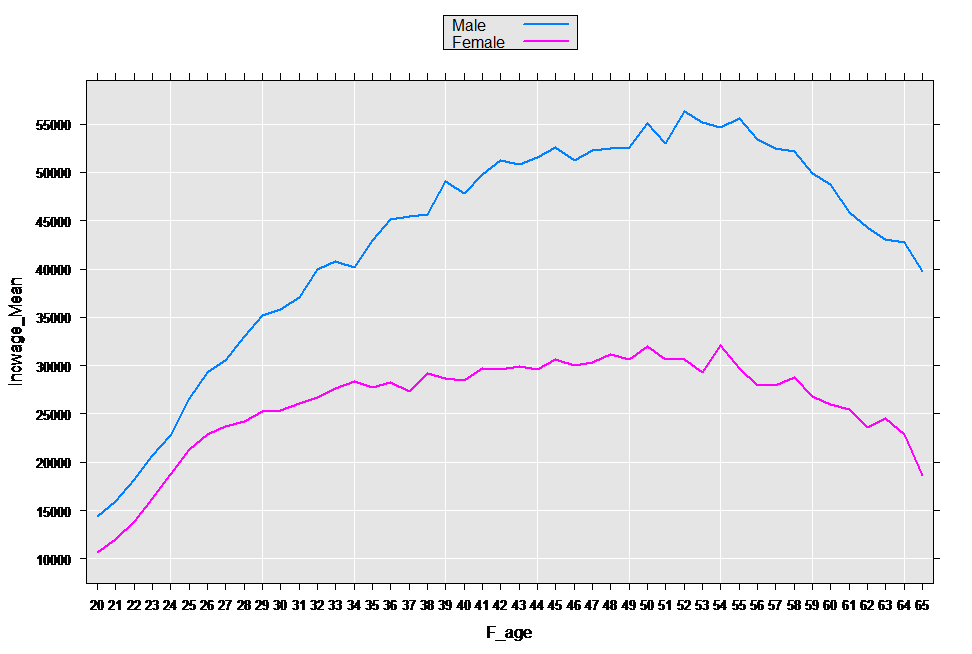
By-group statistics are often computed for further analysis or plotting. It can be convenient to store these results in a .xdf file, especially when there are a large number of groups. In this example, compute the mean and standard deviation of wage income and number of weeks work for each year of age for both men and women using the CensusWorkers.xdf file with data from three states:
# Writing By-Group Summary Statistics to an .xdf File

readPath <- rxGetOption("sampleDataDir")
censusWorkers <- file.path(readPath, "CensusWorkers.xdf")
rxSummary(~ incwage:F(age):sex + wkswork1:F(age):sex, data = censusWorkers,
	byGroupOutFile = "ByAge.xdf",
	summaryStats = c("Mean", "StdDev", "SumOfWeights"),
	pweights = "perwt", overwrite = TRUE)
Results
Call:
rxSummary(formula = ~incwage:F(age):sex + wkswork1:F(age):sex,
	data = censusWorkers, byGroupOutFile = "ByAge.xdf", summaryStats = c("Mean",
		"StdDev", "SumOfWeights"), pweights = "perwt", overwrite = TRUE)

Summary Statistics Results for: ~incwage:F(age):sex + wkswork1:F(age):sex
Data: censusWorkers (RxXdfData Data Source)
File name: C:/Program Files/Microsoft/ML Server/R_SERVER/library/RevoScaleR/SampleData/CensusWorkers.xdf
Probability weights: perwt
Number of valid observations: 351121

	Name               Mean       StdDev      SumOfWeights
	incwage:F_age:sex  35788.4675 40605.12565 7143286
	wkswork1:F_age:sex    48.6373     6.94423 7143286

By-group statistics for incwage:F(age):sex contained in C:\YourDir\ByAge.xdf
By-group statistics for wkswork1:F(age):sex contained in C:\YourDir\ByAge.xdf
You can take a quick look at the first five rows in the data set to see that the first variables are the two factor variables determining the groups: F_age and sex. The remaining variables are the computed by-group statistics.
rxGetInfo("ByAge.xdf", numRows = 5)
Results
File name: C:\YourDir\ByAge.xdf
Number of observations: 92
Number of variables: 8
Number of blocks: 1
Compression type: zlib
Data (5 rows starting with row 1):
	F_age  sex incwage_Mean incwage_StdDev incwage_SumOfWeights wkswork1_Mean
1    20 Male     14437.68       14118.49                71089      44.29758
2    21 Male     15981.48       13191.73                71150      45.27770
3    22 Male     18258.04       13919.44                75979      46.07166
4    23 Male     20739.91       16511.88                79663      46.75025
5    24 Male     22737.17       15345.41                81412      47.51487
	wkswork1_StdDev wkswork1_SumOfWeights
1        9.755092                 71089
2        9.110743                 71150
3        8.903617                 75979
4        8.451298                 79663
5        7.942226                 81412
You can plot directly from the .xdf file to visualize the results:
rxLinePlot(incwage_Mean~F_age, groups = sex, data = "ByAge.xdf")
Transform data in-flight
You can use the transforms argument to modify your data set before computing a summary. When used in this way, the original data is unmodified and no permanent copy of the modified data is written to disk. The data summaries returned, however, reflect the modified data.
You can also transform data in the formula itself, by specifying simple functions of the original variables. For example, you can get a summary based on the natural logarithm of a variable as follows:
# Transform data in rxSummary
rxSummary(~ log(incwage), data = censusWorkers)
Results
Call:
rxSummary(formula = ~log(incwage), data = censusWorkers)

Summary Statistics Results for: ~log(incwage)
Data: censusWorkers (RxXdfData Data Source)
File name: C:/Program Files/Microsoft/ML Server/R_SERVER/library/RevoScaleR/SampleData/CensusWorkers.xdf
Number of valid observations: 351121

Name         Mean     StdDev    Min      Max      ValidObs MissingObs
log(incwage) 10.19694 0.8387598 1.386294 12.77705 331625   19496
Compute and plot Lorenz curves
The Lorenz curves were originally developed to illustrate income inequality. For example, it can show us what percentage of total income is attributed to the lowest earning 10% of the population. The rxLorenz function from RevoScaleR provides a "big data" version, using approximate quantiles to quickly compute the cumulative distribution by quantile in a single pass through the data.
The rxLorenz function requires an orderVarName, the name of the variable used to compute the quantiles. A separate valueVarName can also be specified. This is the name of the variable used to compute the mean values by quantile. By default, the same variable is used for both. We can continue to use the Census Workers data set as an example, computing a Lorenz curve for the distribution of income:
lorenzOut <- rxLorenz(orderVarName = "incwage", data = censusWorkers,
	pweights = "perwt")
head(lorenzOut)

	cumVals  percents
1 0.0000000  0.000000
2 0.3642878  9.126934
3 0.4005827  9.363072
4 0.5368416 10.181295
5 0.5666976 10.353428
6 0.6241598 10.667766
The returned object contains the cumulative values and the percentages. Using the plot method for rxLorenz, we can get a visual representation of the income distribution and compare it with the horizontal line representing perfect equality:
plot(lorenzOut)
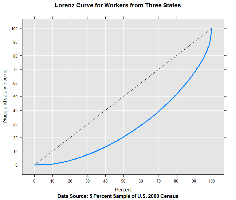
The Gini coefficient is often used as a summary statistic for Lorenz curves. It is computed by estimating the ratio of the area between the line of equality and the Lorenz curve to the total area under the line of equality (using trapezoidal integration). The Gini coefficient can range from 0 to 1, with 0 representing perfect equality. We can compute it from using the output from rxLorenz:
giniCoef <- rxGini(lorenzOut)
giniCoef

	[1] 0.4491421
Tips for wide data sets
Building a better understanding of the distribution of each variable and the relationships between variables improves decision making during the modeling phase. This is especially true for wide data sets containing hundreds if not thousands of variables. For wide data sets, the main goal of data exploration should be to find any outliers or influential data points, identify redundant variables or correlated variables and transform or combine any variables that seem appropriate.
The functions rxGetVarInfo and rxSummary provide useful information can help in this effort, but these two functions may need to be used differently when the data contain many variables.
As a first step, import the data to an .xdf so that you can execute functions providing metadata and summary statistics. Recall that rxGetVarInfo returns metadata about the data object. After loading data into an XDF data source, the data type information can easily be accessed using the rxGetVarInfo function.
Because wide data has so many variables, printed output can be hard to read. As an alternative, save the variable information to an object that can serve as in informal data dictionary. We demonstrate this using the Claims data from the sample data directory:
readPath <- rxGetOption("sampleDataDir")
censusWorkers <- file.path(readPath, "CensusWorkers.xdf")
censusDataDictionary <-rxGetVarInfo(censusWorkers)
We can then obtain the information for an individual variable as follows:
censusDataDictionary$age

Age
		Type: integer, Low/High: (20, 65)
The rxSummary function is a great way to look at the distribution of individual variables and identify outliers. With wide data, you want to store the results of this function into an object. This object contains a data frame with the results of the numeric variables, “sDataFrame”, and a list of data frames with the counts for each categorical variable,”categorical”:
readPath <- rxGetOption("sampleDataDir")
censusWorkers <- file.path(readPath, "CensusWorkers.xdf")
censusSummary <- rxSummary(~ age + incwage + perwt + sex + wkswork1,
	data = censusWorkers)
names(censusSummary)

[1] "nobs.valid"       "nobs.missing"     "sDataFrame"       "categorical"
[5] "params"           "formula"          "call"             "categorical.type"
Printing the rxSummary results to the console wouldn’t be useful with so many variables. Saving the results in an object allows us to not only access the summary results programmatically, but also to view the results separately for numeric and categorical variables. We access the sDataFrame (printed to show structure) as follows:
censusSummary$sDataFrame
		Name        Mean       StdDev Min    Max ValidObs MissingObs
1      age    40.42814    11.385017  20     65   351121          0
2  incwage 35333.83894 40444.544084   0 354000   351121          0
3    perwt    20.34423     9.633100   2    168   351121          0
4      sex          NA           NA  NA     NA   351121          0
5 wkswork1    48.62566     6.953843  21     52   351121          0
To view the categorical variables, we access the categorical component:
censusSummary$categorical
[[1]]
		sex Counts
1   Male 189344
2 Female 161777
Another key piece of data exploration for wide data is looking at the relationships between variables to find variables that are measuring the same information or variables that are correlated. With variables that are measuring the same information, perhaps one stands out as being representative of the group. During data exploration, you must rely on your domain knowledge to group variables into related sets or prioritize variables that are important based on the field or industry. Paring the data set down to related sets allow you to look more closely at redundancy and relatedness within each set.
When looking for correlation between variables the function rxCrosstabs is useful. In Crosstabs, you see how to use rxCrosstabs and rxLinePlot to graph the relationship between two variables. Graphs allow for a quick view of the relationship between two variables, which comes in handy when you have many variables to consider. For more information, see Visualizing Huge Data Sets: An Example from the U.S. Census.