将条件格式应用于特定 Excel 范围

Excel JavaScript 库提供了用于将条件格式应用于工作表中的特定数据范围的 API。 借助此功能，可以轻松直观地解析大型数据集。 该格式还会基于相应范围内的更改进行动态更新。

注意

本文介绍了 Excel JavaScript 外接程序上下文中的条件格式。下面的文章提供了有关在 Excel 中实现完整条件格式功能的详细信息。

• 添加、更改或清除条件格式
• 将公式用于条件格式

条件格式的编程控制

Range.conditionalFormats 属性是一个应用于相应范围的 ConditionalFormat 对象的集合。 ConditionalFormat 对象包含多个属性，这些属性基于 ConditionalFormatType 定义要应用的格式。

• cellValue
• colorScale
• custom
• dataBar
• iconSet
• preset
• textComparison
• topBottom

注意

每个格式属性都有相应的 *OrNullObject 变体。 在 *OrNullObject 方法部分中了解有关该模式的更多信息。

仅可为 ConditionalFormat 对象设置一种格式类型。 该格式类型由 type 属性确定，该属性是 ConditionalFormatType 枚举值。 type 是在向某一范围添加条件格式时设置的。

创建条件格式规则

条件格式可通过使用 conditionalFormats.add 添加到某一范围。 添加后，可以设置特定于条件格式的属性。 以下示例展示了如何创建不同的格式类型。

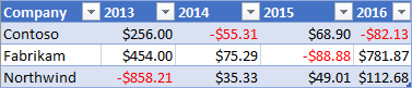
单元格值

单元格值条件格式将基于 ConditionalCellValueRule 中的一个或两个公式的结果应用用户定义的格式。 operator 属性是一个 ConditionalCellValueOperator，用于定义结果表达式与格式设置的关系。

以下示例展示的是将红色字体颜色设置应用于相应范围内小于零的任何值。

await Excel.run(async (context) => {
    const sheet = context.workbook.worksheets.getItem("Sample");
    const range = sheet.getRange("B21:E23");
    const conditionalFormat = range.conditionalFormats.add(
        Excel.ConditionalFormatType.cellValue
    );
    
    // Set the font of negative numbers to red.
    conditionalFormat.cellValue.format.font.color = "red";
    conditionalFormat.cellValue.rule = { formula1: "=0", operator: "LessThan" };
    
    await context.sync();
});

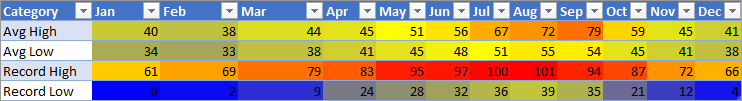
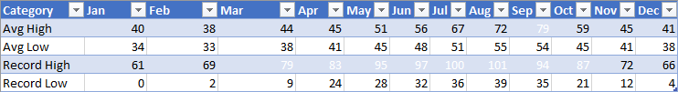
色阶

色阶条件格式可将颜色渐变应用到相应数据范围。 ColorScaleConditionalFormat 上的 criteria 属性定义了三个 ConditionalColorScaleCriterion：minimum、maximum 以及可选的 midpoint。 每个条件色阶点都具有三个属性：

• color - 端点的 HTML 颜色代码。
• formula - 表示端点的数字或公式。 如果 type 是 lowestValue 或 highestValue，该属性将为 null。
• type - 应如何评估公式。 highestValue 和 lowestValue 是指将要应用格式的范围中的值。

下面的示例展示了一个使用蓝色、黄色和红色颜色渐变的范围。 请注意，minimum 和 maximum 分别是最低值和最高值，并使用了 null 公式。 midpoint 使用的类型为 percentage，公式为 "=50"，因此颜色最黄的单元格是平均值。

await Excel.run(async (context) => {
    const sheet = context.workbook.worksheets.getItem("Sample");
    const range = sheet.getRange("B2:M5");
    const conditionalFormat = range.conditionalFormats.add(
          Excel.ConditionalFormatType.colorScale
    );
    
    // Color the backgrounds of the cells from blue to yellow to red based on value.
    const criteria = {
          minimum: {
               formula: null,
               type: Excel.ConditionalFormatColorCriterionType.lowestValue,
               color: "blue"
          },
          midpoint: {
               formula: "50",
               type: Excel.ConditionalFormatColorCriterionType.percent,
               color: "yellow"
          },
          maximum: {
               formula: null,
               type: Excel.ConditionalFormatColorCriterionType.highestValue,
               color: "red"
          }
    };
    conditionalFormat.colorScale.criteria = criteria;
    
    await context.sync();
});

自定义

自定义条件格式根据任意复杂度的公式将用户定义的格式应用于单元格。 ConditionalFormatRule 对象允许使用不同表示法定义公式：

• formula - 标准表示法。
• formulaLocal - 基于用户语言进行本地化。
• formulaR1C1 - R1C1 样式表示法。

在下面的示例中，将数值大于其左侧单元格数值的单元格的字体颜色设置成了绿色。

await Excel.run(async (context) => {
    const sheet = context.workbook.worksheets.getItem("Sample");
    const range = sheet.getRange("B8:E13");
    const conditionalFormat = range.conditionalFormats.add(
         Excel.ConditionalFormatType.custom
    );
    
    // If a cell has a higher value than the one to its left, set that cell's font to green.
    conditionalFormat.custom.rule.formula = '=IF(B8>INDIRECT("RC[-1]",0),TRUE)';
    conditionalFormat.custom.format.font.color = "green";
    
    await context.sync();
});

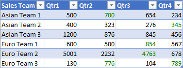
数据栏

数据栏条件格式可将数据栏添加到单元格。 默认情况下，相应范围内的最小和最大值形成数据栏的边界和比例大小。 对象 DataBarConditionalFormat 具有多个属性来控制条形图的外观。

下面的示例对相应范围应用了从左到右填充的数据栏格式。

await Excel.run(async (context) => {
    const sheet = context.workbook.worksheets.getItem("Sample");
    const range = sheet.getRange("B8:E13");
    const conditionalFormat = range.conditionalFormats.add(
         Excel.ConditionalFormatType.dataBar
    );
    
    // Give left-to-right, default-appearance data bars to all the cells.
    conditionalFormat.dataBar.barDirection = Excel.ConditionalDataBarDirection.leftToRight;
    await context.sync();
});

图标集

图标集条件格式使用 Excel 图标来突出显示单元格。 criteria 属性是一个 ConditionalIconCriterion 数组，它定义要插入的符号以及插入该符号的条件。 此数组将使用具有默认属性的条件元素自动预填充。 个别属性不能被覆盖。 相反，必须替换整个条件对象。

下面的示例展示了应用于相应范围的三元素图标集。

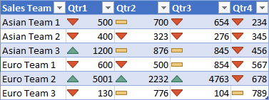
await Excel.run(async (context) => {
    const sheet = context.workbook.worksheets.getItem("Sample");
    const range = sheet.getRange("B8:E13");
    const conditionalFormat = range.conditionalFormats.add(
         Excel.ConditionalFormatType.iconSet
    );
    
    const iconSetCF = conditionalFormat.iconSet;
    iconSetCF.style = Excel.IconSet.threeTriangles;
    
    /*
       With a "three*" icon set style, such as "threeTriangles", the third
        element in the criteria array (criteria[2]) defines the "top" icon;
        e.g., a green triangle. The second (criteria[1]) defines the "middle"
        icon, The first (criteria[0]) defines the "low" icon, but it can often 
        be left empty as this method does below, because every cell that
       does not match the other two criteria always gets the low icon.
    */
    iconSetCF.criteria = [
        {},
          {
            type: Excel.ConditionalFormatIconRuleType.number,
            operator: Excel.ConditionalIconCriterionOperator.greaterThanOrEqual,
            formula: "=700"
          },
          {
            type: Excel.ConditionalFormatIconRuleType.number,
            operator: Excel.ConditionalIconCriterionOperator.greaterThanOrEqual,
            formula: "=1000"
          }
    ];

    await context.sync();
});

预设条件

预设条件格式会基于所选标准规则将用户定义的格式应用于相应范围。 这些规则由 ConditionalPresetCriteriaRule 中的 ConditionalFormatPresetCriterion 定义。

以下示例将字体设置为白色，只要单元格的值至少高于该范围的平均值一个标准偏差。

await Excel.run(async (context) => {
    const sheet = context.workbook.worksheets.getItem("Sample");
    const range = sheet.getRange("B2:M5");
    const conditionalFormat = range.conditionalFormats.add(
         Excel.ConditionalFormatType.presetCriteria
    );
    
    // Color every cell's font white that is one standard deviation above average relative to the range.
    conditionalFormat.preset.format.font.color = "white";
    conditionalFormat.preset.rule = {
         criterion: Excel.ConditionalFormatPresetCriterion.oneStdDevAboveAverage
    };
    
    await context.sync();
});

文本比较

文本比较条件格式将字符串比较作为条件。 rule 属性是一个 ConditionalTextComparisonRule，用于定义要与单元格进行比较的字符串，以及用于指定比较类型的运算符。

以下示例在单元格的文本包含“Delayed”时将字体颜色设置为红色。

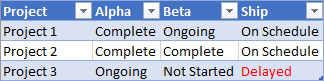
await Excel.run(async (context) => {
    const sheet = context.workbook.worksheets.getItem("Sample");
    const range = sheet.getRange("B16:D18");
    const conditionalFormat = range.conditionalFormats.add(
         Excel.ConditionalFormatType.containsText
    );
    
    // Color the font of every cell containing "Delayed".
    conditionalFormat.textComparison.format.font.color = "red";
    conditionalFormat.textComparison.rule = {
         operator: Excel.ConditionalTextOperator.contains,
         text: "Delayed"
    };
    
    await context.sync();
});

顶/底

顶/底条件格式将格式应用于相应范围中的最高值或最低值。 rule 属性的类型为 ConditionalTopBottomRule，用于设置条件是基于最高还是最低，以及评估是基于排名还是基于百分比。

在下面的示例中，向相应范围中的最高值单元格应用了绿色突出显示。

await Excel.run(async (context) => {
    const sheet = context.workbook.worksheets.getItem("Sample");
    const range = sheet.getRange("B21:E23");
    const conditionalFormat = range.conditionalFormats.add(
         Excel.ConditionalFormatType.topBottom
    );
    
    // For the highest valued cell in the range, make the background green.
    conditionalFormat.topBottom.format.fill.color = "green"
    conditionalFormat.topBottom.rule = { rank: 1, type: "TopItems"}
    
    await context.sync();
});

更改条件格式规则

对象 ConditionalFormat 提供了多种方法，用于在设置条件格式规则后更改这些规则。

• changeRuleToCellValue
• changeRuleToColorScale
• changeRuleToContainsText
• changeRuleToCustom
• changeRuleToDataBar
• changeRuleToIconSet
• changeRuleToPresetCriteria
• changeRuleToTopBottom

以下示例演示如何使用 changeRuleToPresetCriteria 上述列表中的 方法将现有条件格式规则更改为预设条件规则类型。

注意

指定的区域必须具有现有的条件格式规则才能使用更改方法。 如果指定的区域没有条件格式规则，则更改方法不会应用新规则。

await Excel.run(async (context) => {
    const sheet = context.workbook.worksheets.getItem("Sample");
    const range = sheet.getRange("B2:M5");
    
    // Retrieve the first existing `ConditionalFormat` rule on this range. 
    // Note: The specified range must have an existing conditional format rule.
    const conditionalFormat = range.conditionalFormats.getItemOrNullObject("0");
    
    // Change the conditional format rule to preset criteria.
    conditionalFormat.changeRuleToPresetCriteria({
        criterion: Excel.ConditionalFormatPresetCriterion.oneStdDevAboveAverage, 
    });
    conditionalFormat.preset.format.font.color = "red";
    
    await context.sync();
});

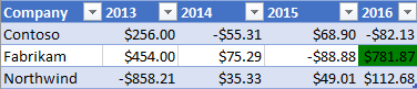
多种格式和优先级

你可以将多个条件格式应用于某一范围。 如果这些格式具有冲突的元素，例如不同的字体颜色，则只有一种格式会应用该特定元素。 优先级由 ConditionalFormat.priority 属性定义。 优先级是一个数字（等于 ConditionalFormatCollection 中的索引），可在创建格式时设置。 值越小 priority ，格式的优先级越高。

以下示例展示了两种格式之间存在冲突时的字体颜色选择。 负数将被设置为粗体字体，但不会被设置为红色字体，因为将其设置为蓝色字体的格式具有更高的优先级。

await Excel.run(async (context) => {
    const sheet = context.workbook.worksheets.getItem("Sample");
    const temperatureDataRange = sheet.tables.getItem("TemperatureTable").getDataBodyRange();
    
    
    // Set low numbers to bold, dark red font and assign priority 1.
    const presetFormat = temperatureDataRange.conditionalFormats
        .add(Excel.ConditionalFormatType.presetCriteria);
    presetFormat.preset.format.font.color = "red";
    presetFormat.preset.format.font.bold = true;
    presetFormat.preset.rule = { criterion: Excel.ConditionalFormatPresetCriterion.oneStdDevBelowAverage };
    presetFormat.priority = 1;
    
    // Set negative numbers to blue font with green background and set priority 0.
    const cellValueFormat = temperatureDataRange.conditionalFormats
        .add(Excel.ConditionalFormatType.cellValue);
    cellValueFormat.cellValue.format.font.color = "blue";
    cellValueFormat.cellValue.format.fill.color = "lightgreen";
    cellValueFormat.cellValue.rule = { formula1: "=0", operator: "LessThan" };
    cellValueFormat.priority = 0;
    
    await context.sync();
});

互斥条件格式

ConditionalFormat 的 stopIfTrue 属性可防止将较低优先级条件格式应用于相应范围。 如果与条件格式匹配的范围应用了 stopIfTrue === true，则不会再应用后续的条件格式，即使它们的格式细节不冲突。

以下示例展示了正被添加到某一范围的两种条件格式。 无论其他格式条件是否为真，负数都将被设置为具有浅绿色背景的蓝色字体。

await Excel.run(async (context) => {
    const sheet = context.workbook.worksheets.getItem("Sample");
    const temperatureDataRange = sheet.tables.getItem("TemperatureTable").getDataBodyRange();
    
    // Set low numbers to bold, dark red font and assign priority 1.
    const presetFormat = temperatureDataRange.conditionalFormats
        .add(Excel.ConditionalFormatType.presetCriteria);
    presetFormat.preset.format.font.color = "red";
    presetFormat.preset.format.font.bold = true;
    presetFormat.preset.rule = { criterion: Excel.ConditionalFormatPresetCriterion.oneStdDevBelowAverage };
    presetFormat.priority = 1;
    
    // Set negative numbers to blue font with green background and 
    // set priority 0, but set stopIfTrue to true, so none of the 
    // formatting of the conditional format with the higher priority
    // value will apply, not even the bolding of the font.
    const cellValueFormat = temperatureDataRange.conditionalFormats
        .add(Excel.ConditionalFormatType.cellValue);
    cellValueFormat.cellValue.format.font.color = "blue";
    cellValueFormat.cellValue.format.fill.color = "lightgreen";
    cellValueFormat.cellValue.rule = { formula1: "=0", operator: "LessThan" };
    cellValueFormat.priority = 0;
    cellValueFormat.stopIfTrue = true;
    
    await context.sync();
});

清除条件格式规则

若要从特定条件格式规则中删除格式属性，请使用 对象的 clearFormat 方法 ConditionalRangeFormat 。 方法 clearFormat 创建不带格式设置的格式设置规则。

若要从特定区域或整个工作表中删除所有条件格式规则，请使用 对象的 clearAll 方法 ConditionalFormatCollection 。

下面的示例演示如何使用 clearAll 方法从工作表中删除所有条件格式。

await Excel.run(async (context) => {
    const sheet = context.workbook.worksheets.getItem("Sample");
    const range = sheet.getRange();
    range.conditionalFormats.clearAll();

    await context.sync();
});

另请参阅

• Excel 加载项中的 Word JavaScript 对象模型
• ConditionalFormat 对象（适用于 Excel 的 JavaScript API）
• 添加、更改或清除条件格式
• 将公式用于条件格式