教學課程：使用自動化機器學習在 Python 中定型模型

發行項
03/10/2024

Azure 機器學習是雲端式環境，可讓您定型、部署、自動化、管理和追蹤機器學習模型。

在本教學課程中，您會在 Azure 機器學習中使用自動化機器學習來建立回歸模型來預測計程車車資價格。此程式會接受定型數據和組態設定，並自動逐一查看不同方法、模型和超參數設定的組合，以達到最佳模型。

在本教學課程中，您會了解如何：

使用 Apache Spark 和 Azure 開放數據集下載數據。
使用 Apache Spark DataFrame 轉換和清除數據。
在自動化機器學習中定型回歸模型。
計算模型精確度。

開始之前

警告

自 2023 年 9 月 29 日起，Azure Synapse 將會停止對 Spark 2.4 運行時間的官方支援。在 2023 年 9 月 29 日之後，我們不會處理任何與 Spark 2.4 相關的支援票證。 Spark 2.4 的 Bug 或安全性修正不會有發行管線。使用Spark 2.4後，支援截止日期會自行承擔風險。由於潛在的安全性和功能考慮，我們強烈勸阻其繼續使用。
作為 Apache Spark 2.4 淘汰程式的一部分，我們想要通知您 Azure Synapse Analytics 中的 AutoML 也將已被取代。這包括低程式代碼介面和用來透過程式代碼建立 AutoML 試用版的 API。
請注意，AutoML 功能是透過 Spark 2.4 運行時間獨佔提供的。
對於想要繼續使用 AutoML 功能的客戶，建議您將資料儲存到 Azure Data Lake 儲存體 Gen2 （ADLSg2）帳戶。您可以從該處順暢地透過 Azure 機器學習（AzureML）存取 AutoML 體驗。如需此因應措施的詳細資訊，請參閱這裡。

了解回歸模型

回歸模型 會根據獨立預測值預測數值。在回歸中，目標是藉由估計一個變數如何影響其他變數，協助建立這些獨立預測變數之間的關聯性。

以紐約市計程車數據為基礎的範例

在此範例中，您會使用Spark對紐約市（NYC）的計程車車程小費數據執行一些分析。數據可透過 Azure 開放資料集取得。此數據集子集包含黃色計程車車程的相關信息，包括每個車程的相關信息、開始和結束時間和位置，以及成本。

重要

從其儲存位置提取此數據可能會產生額外費用。在下列步驟中，您會開發模型來預測 NYC 計程車車資價格。

下載並準備數據

方法如下：

使用 PySpark 核心建立筆記本。如需指示，請參閱建立筆記本。

注意

由於使用 PySpark 核心，因此不需要明確建立任何內容。當您執行第一個程式代碼數據格時，系統會自動為您建立Spark內容。

由於原始數據採用 Parquet 格式，因此您可以使用 Spark 內容，將檔案直接提取到記憶體中做為 DataFrame。透過開放式數據集 API 擷取數據來建立 Spark 數據框架。在這裡，您可以使用Spark DataFrame schema on read 屬性來推斷數據類型和架構。

blob_account_name = "azureopendatastorage"
blob_container_name = "nyctlc"
blob_relative_path = "yellow"
blob_sas_token = r""

# Allow Spark to read from the blob remotely
wasbs_path = 'wasbs://%s@%s.blob.core.windows.net/%s' % (blob_container_name, blob_account_name, blob_relative_path)
spark.conf.set('fs.azure.sas.%s.%s.blob.core.windows.net' % (blob_container_name, blob_account_name),blob_sas_token)

# Spark read parquet; note that it won't load any data yet
df = spark.read.parquet(wasbs_path)

視 Spark 集區的大小而定，原始數據可能太大或需要太多時間才能運作。您可以使用和 end_date 篩選，將此數據篩選為較小的專案，例如一個月的數據start_date。篩選 DataFrame 之後，您也會在新 DataFrame 上執行函 describe() 式，以查看每個欄位的摘要統計數據。

根據摘要統計數據，您可以看到數據中有一些不規則。例如，統計數據顯示最小車程距離小於0。您需要篩選掉這些不規則的數據點。
```
# Create an ingestion filter
start_date = '2015-01-01 00:00:00'
end_date = '2015-12-31 00:00:00'

filtered_df = df.filter('tpepPickupDateTime > "' + start_date + '" and tpepPickupDateTime< "' + end_date + '"')

filtered_df.describe().show()
```

從數據集產生特徵，方法是選取一組數據行，並從取貨 datetime 欄位建立各種以時間為基礎的功能。篩選出先前步驟中識別的極端值，然後移除最後幾個數據行，因為它們不需要定型。

from datetime import datetime
from pyspark.sql.functions import *

# To make development easier, faster, and less expensive, downsample for now
sampled_taxi_df = filtered_df.sample(True, 0.001, seed=1234)

taxi_df = sampled_taxi_df.select('vendorID', 'passengerCount', 'tripDistance',  'startLon', 'startLat', 'endLon' \
                                , 'endLat', 'paymentType', 'fareAmount', 'tipAmount'\
                                , column('puMonth').alias('month_num') \
                                , date_format('tpepPickupDateTime', 'hh').alias('hour_of_day')\
                                , date_format('tpepPickupDateTime', 'EEEE').alias('day_of_week')\
                                , dayofmonth(col('tpepPickupDateTime')).alias('day_of_month')
                                ,(unix_timestamp(col('tpepDropoffDateTime')) - unix_timestamp(col('tpepPickupDateTime'))).alias('trip_time'))\
                        .filter((sampled_taxi_df.passengerCount > 0) & (sampled_taxi_df.passengerCount < 8)\
                                & (sampled_taxi_df.tipAmount >= 0)\
                                & (sampled_taxi_df.fareAmount >= 1) & (sampled_taxi_df.fareAmount <= 250)\
                                & (sampled_taxi_df.tipAmount < sampled_taxi_df.fareAmount)\
                                & (sampled_taxi_df.tripDistance > 0) & (sampled_taxi_df.tripDistance <= 200)\
                                & (sampled_taxi_df.rateCodeId <= 5)\
                                & (sampled_taxi_df.paymentType.isin({"1", "2"})))
taxi_df.show(10)

如您所見，這會建立新的 DataFrame，其中包含月份當天、取貨時間、工作日和總車程時間的其他數據行。

Picture of taxi DataFrame.

產生測試和驗證數據集

擁有最終數據集之後，您可以使用 Spark 中的函式，將數據分割成定型和測試集 random_ split 。藉由使用提供的權數，此函式會隨機將數據分割成用於模型定型的定型數據集，以及用於測試的驗證數據集。

# Random split dataset using Spark; convert Spark to pandas
training_data, validation_data = taxi_df.randomSplit([0.8,0.2], 223)

此步驟可確保測試已完成模型的數據點尚未用來定型模型。

連線至 Azure 機器學習工作區

在 Azure 機器學習中，工作區是接受 Azure 訂用帳戶和資源資訊的類別。它也會建立雲端資源來監視和追蹤您的模型執行。在此步驟中，您會從現有的 Azure 機器學習工作區建立工作區物件。

from azureml.core import Workspace

# Enter your subscription id, resource group, and workspace name.
subscription_id = "<enter your subscription ID>" #you should be owner or contributor
resource_group = "<enter your resource group>" #you should be owner or contributor
workspace_name = "<enter your workspace name>" #your workspace name

ws = Workspace(workspace_name = workspace_name,
               subscription_id = subscription_id,
               resource_group = resource_group)

將 DataFrame 轉換成 Azure 機器學習數據集

若要提交遠程實驗，請將數據集轉換成 Azure 機器學習 TabularDatset 實例。 TabularDataset 藉由剖析提供的檔案，以表格式表示數據。

下列程式代碼會取得現有的工作區和預設 Azure 機器學習資料存放區。然後，它會將數據存放區和檔案位置傳遞至 path 參數，以建立新的 TabularDataset 實例。

import pandas 
from azureml.core import Dataset

# Get the Azure Machine Learning default datastore
datastore = ws.get_default_datastore()
training_pd = training_data.toPandas().to_csv('training_pd.csv', index=False)

# Convert into an Azure Machine Learning tabular dataset
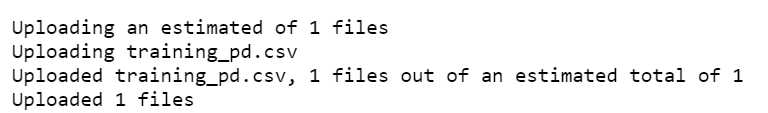
datastore.upload_files(files = ['training_pd.csv'],
                       target_path = 'train-dataset/tabular/',
                       overwrite = True,
                       show_progress = True)
dataset_training = Dataset.Tabular.from_delimited_files(path = [(datastore, 'train-dataset/tabular/training_pd.csv')])

Picture of uploaded dataset.

提交自動化實驗

下列各節將逐步引導您完成提交自動化機器學習實驗的程式。

定義定型設定

若要提交實驗，您必須定義定型的實驗參數和模型設定。如需設定的完整清單，請參閱在 Python 中設定自動化機器學習實驗。

import logging

automl_settings = {
    "iteration_timeout_minutes": 10,
    "experiment_timeout_minutes": 30,
    "enable_early_stopping": True,
    "primary_metric": 'r2_score',
    "featurization": 'auto',
    "verbosity": logging.INFO,
    "n_cross_validations": 2}

將定義的定型設定當做 kwargs 參數傳遞至 AutoMLConfig 物件。因為您使用 Spark，因此您也必須傳遞 Spark 內容，變數會自動存取 sc 此內容。此外，您可以指定定型數據和模型類型，在此案例中為回歸。

from azureml.train.automl import AutoMLConfig

automl_config = AutoMLConfig(task='regression',
                             debug_log='automated_ml_errors.log',
                             training_data = dataset_training,
                             spark_context = sc,
                             model_explainability = False, 
                             label_column_name ="fareAmount",**automl_settings)

注意

自動化機器學習前置處理步驟會成為基礎模型的一部分。這些步驟包括功能正規化、處理遺漏的數據，以及將文字轉換成數值。當您使用模型進行預測時，定型期間套用的相同前置處理步驟會自動套用至您的輸入數據。

定型自動回歸模型

接下來，您會在 Azure 機器學習工作區中建立實驗物件。實驗可作為個別執行的容器。

from azureml.core.experiment import Experiment

# Start an experiment in Azure Machine Learning
experiment = Experiment(ws, "aml-synapse-regression")
tags = {"Synapse": "regression"}
local_run = experiment.submit(automl_config, show_output=True, tags = tags)

# Use the get_details function to retrieve the detailed output for the run.
run_details = local_run.get_details()

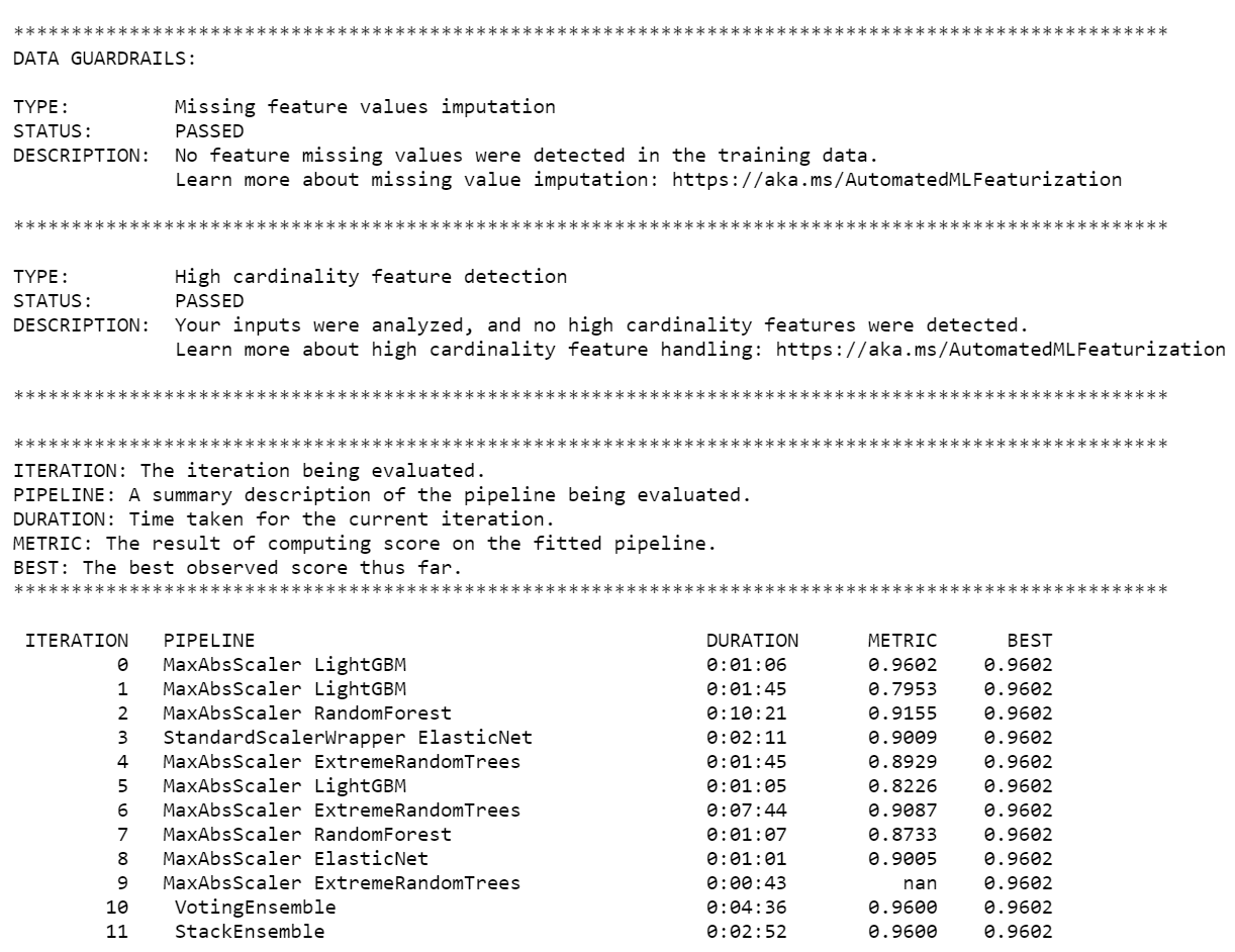
實驗完成時，輸出會傳回已完成反覆專案的詳細數據。針對每個反覆專案，您會看到模型類型、執行持續時間和定型精確度。欄位會 BEST 根據您的計量類型追蹤最佳執行訓練分數。

Screenshot of model output.

注意

提交自動化機器學習實驗之後，它會執行各種反覆專案和模型類型。此執行通常需要 60 到 90 分鐘。

擷取最佳模型

若要從反覆項目選取最佳模型，請使用函 get_output 式傳回最佳的執行和配適模型。下列程式代碼會擷取任何已記錄計量或特定反覆專案的最佳執行和配適模型。

# Get best model
best_run, fitted_model = local_run.get_output()

測試模型精確度

若要測試模型精確度，請使用最佳模型在測試數據集上執行計程車車資預測。函 predict 式會使用最佳模型，並從驗證數據集預測（費用金額）的值 y 。
```
# Test best model accuracy
validation_data_pd = validation_data.toPandas()
y_test = validation_data_pd.pop("fareAmount").to_frame()
y_predict = fitted_model.predict(validation_data_pd)
```
根平均平方誤差是模型所預測樣本值與觀察到值之間差異的常用量值。藉由比較 y_test DataFrame 與模型預測的值，即可計算結果的根平均平方誤差。

函式 mean_squared_error 會採用兩個陣列，並計算它們之間的平均平方誤差。然後，您會取得結果的平方根。此計量大致表示計程車車資預測與實際車資值相距甚遠。
```
from sklearn.metrics import mean_squared_error
from math import sqrt

# Calculate root-mean-square error
y_actual = y_test.values.flatten().tolist()
rmse = sqrt(mean_squared_error(y_actual, y_predict))

print("Root Mean Square Error:")
print(rmse)
```
```
Root Mean Square Error:
2.309997102577151
```
根平均平方誤差是模型預測響應精確度的良好量值。從結果中，您會看到模型相當擅長從數據集特徵預測計程車車資，通常是在 $2.00 內。

執行下列程式代碼來計算平均絕對百分比錯誤。此計量會將精確度表示為錯誤的百分比。其方式是計算每個預測和實際值之間的絕對差異，然後加總所有差異。然後，它會以實際值總數的百分比表示該總和。

# Calculate mean-absolute-percent error and model accuracy 
sum_actuals = sum_errors = 0

for actual_val, predict_val in zip(y_actual, y_predict):
    abs_error = actual_val - predict_val
    if abs_error < 0:
        abs_error = abs_error * -1

    sum_errors = sum_errors + abs_error
    sum_actuals = sum_actuals + actual_val

mean_abs_percent_error = sum_errors / sum_actuals

print("Model MAPE:")
print(mean_abs_percent_error)
print()
print("Model Accuracy:")
print(1 - mean_abs_percent_error)

Model MAPE:
0.03655071038487368

Model Accuracy:
0.9634492896151263

從兩個預測精確度計量中，您會看到模型相當善於從數據集的功能預測計程車費用。

調整線性回歸模型之後，您現在必須判斷模型符合數據的方式。若要這樣做，您會根據預測的輸出繪製實際費用值。此外，您可以計算 R 平方量值，以了解數據與配適回歸線有多接近。

import matplotlib.pyplot as plt
import numpy as np
from sklearn.metrics import mean_squared_error, r2_score

# Calculate the R2 score by using the predicted and actual fare prices
y_test_actual = y_test["fareAmount"]
r2 = r2_score(y_test_actual, y_predict)

# Plot the actual versus predicted fare amount values
plt.style.use('ggplot')
plt.figure(figsize=(10, 7))
plt.scatter(y_test_actual,y_predict)
plt.plot([np.min(y_test_actual), np.max(y_test_actual)], [np.min(y_test_actual), np.max(y_test_actual)], color='lightblue')
plt.xlabel("Actual Fare Amount")
plt.ylabel("Predicted Fare Amount")
plt.title("Actual vs Predicted Fare Amount R^2={}".format(r2))
plt.show()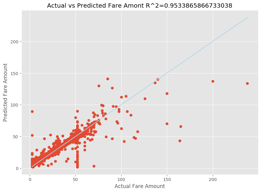

Screenshot of a regression plot.

從結果中，您可以看到 R 平方量值占變數的 95%。這也會由實際繪圖與觀察到的繪圖進行驗證。回歸模型所考慮的變異數越多，數據點越接近適合的回歸線。

向 Azure 機器學習註冊模型

驗證最佳模型之後，您可以將它註冊至 Azure 機器學習。然後，您可以下載或部署已註冊的模型，並接收您註冊的所有檔案。

description = 'My automated ML model'
model_path='outputs/model.pkl'
model = best_run.register_model(model_name = 'NYCYellowTaxiModel', model_path = model_path, description = description)
print(model.name, model.version)

NYCYellowTaxiModel 1

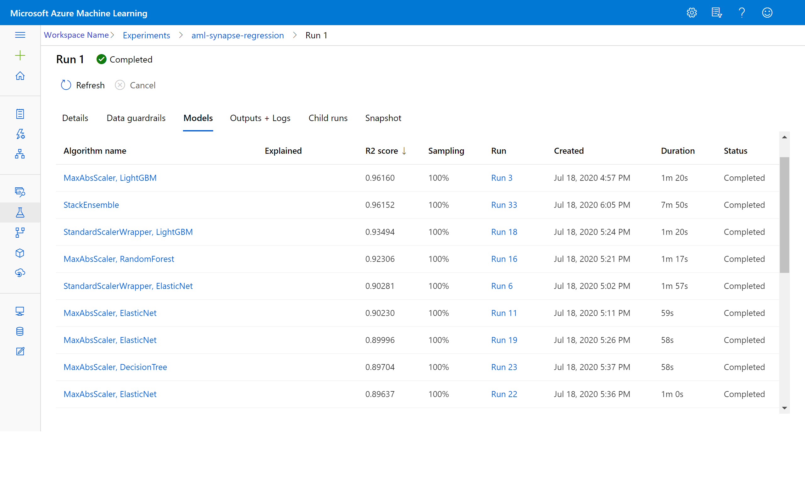
在 Azure 機器學習中檢視結果

您也可以前往 Azure 機器學習工作區中的實驗，以存取反覆項目的結果。您可以在這裡取得執行狀態、嘗試模型和其他模型計量的其他詳細數據。

Screenshot of an Azure Machine Learning workspace.

教學課程：使用自動化機器學習在 Python 中定型模型

開始之前

了解回歸模型

以紐約市計程車數據為基礎的範例

下載並準備數據

產生測試和驗證數據集

連線至 Azure 機器學習工作區

將 DataFrame 轉換成 Azure 機器學習數據集

提交自動化實驗

定義定型設定

定型自動回歸模型

擷取最佳模型

測試模型精確度

向 Azure 機器學習註冊模型

在 Azure 機器學習中檢視結果

下一步

其他資源

教學課程：使用自動化機器學習在 Python 中定型模型

開始之前

了解回歸模型

以紐約市計程車數據為基礎的範例

下載並準備數據

產生測試和驗證數據集

連線 至 Azure 機器學習 工作區

將 DataFrame 轉換成 Azure 機器學習 數據集

提交自動化實驗

定義定型設定

定型自動回歸模型

擷取最佳模型

測試模型精確度

向 Azure 機器學習 註冊模型

在 Azure 機器學習 中檢視結果

下一步

其他資源

連線至 Azure 機器學習工作區

將 DataFrame 轉換成 Azure 機器學習數據集

向 Azure 機器學習註冊模型

在 Azure 機器學習中檢視結果