Tutorial 2

Table of Contents

• Introduction
• The MNIST Data
  • Getting the Data
• Some Important CNTK Concepts
  • CNTK Functions
  • Model Editing
• Starting Shallow: One Hidden Layer Neural Network
  • Neural Network vs. Softmax Regression
  • The Network Definition
  • SGD Parameters
  • Putting it all Together
• Going Deep: Convolutional Neural Networks (CNNs)
  • CNNs: The Ingredients
  • The Network Definition
  • Putting it all Together
• Improving Training: CNN with Batch Normalization
  • Batch Normalization in a Nutshell
  • The Network Definition
  • Putting it all Together

Introduction

This tutorial is for BrainScript. For Python click here. This is the second part of the CNTK tutorial where we will start using CNTK more to its full potential. We will go deep! This tutorial assumes that you have already gone through the first part, and thus you are familiar with basic CNTK/ML concepts such as logistic regression and softmax. In the first tutorial we built models to solve simple binary and multi-class classification problems. Though those models achieved good accuracy, they will not perform as well on harder real-world problems. One principal reason is that the decision boundaries between the classes are not typically linear. In this tutorial, we will learn to build more complex models, namely, neural networks and convolutional neural networks. We will build an image classification system using the MNIST dataset as our benchmark.

The files for this tutorial can be found in the source-code distribution under Examples/Image/GettingStarted (GitHub link).

The MNIST Data

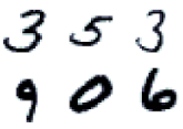
MNIST is a popular image dataset of handwritten digits. It is divided into a training set of 60,000 examples, and a test set of 10,000 examples. This dataset is a subset of the original data from NIST, pre-processed and published by LeCun et al. For more details please refer to this page. The MNIST dataset has become a standard benchmark for machine learning methods because it is real-world data, yet it is simple and requires minimal efforts in pre-processing and formatting. Each instance of the data consists of a 28x28 pixel image representing one digit, with a label between 0 and 9. Here are some examples:

Getting the Data

CNTK comes with a Python script that fetches and prepares the MNIST data for CNTK consumption. You find it here: install_mnist.py.

Some Important CNTK Concepts

Before building the neural networks for written digit image recognition using the MNIST dataset, we will go through two important concepts of CNTK: (1) Functions; and (2) model editing.

CNTK Functions

BrainScript allows user-defined functions. User-defined functions are CNTK's mechanism of creating reusable blocks. Using functions is easy, cuts down on the verbosity of defining networks, increases code re-use, and helps to prevent errors. Using BrainScript's include directive, they can be shared across multiple configuration files. Functions are parameterized expressions. A function's value can be of any type understood by BrainScript, including scalars,

MaxOf (a, b) = if a > b then a else b

nodes of the Computational Network,

# one-liner defining a ReLU unit
RFF (x, W, b) = RectifiedLinear (W * x + b)

and records of values,

RecurrentLSTM (outputDim, x, inputDim) =
[
    # previous values of our outputs h and c below
    dh = PastValue (h)  // h(t-1) 
    dc = PastValue (c)  // c(t-1)

    # functions to define parameters. Each invocation comes with its own set of weights.
    newB() = Parameter (cellDim, 1)         // bias
    newW() = Parameter (cellDim, inputDim)  // input-to-hiden
    newH() = Parameter (cellDim, outputDim) // hidden-to-hidden
    newC() = Parameter (cellDim, 1)         // cell-to-hiddden (elementwise)

    # projections of the LSTM's inputs. Each invocation has its own weights.
    newPIn() = newW() * x + newH() * dh + newB()

    # gates
    i = Sigmoid (newPIn() + newC() .* dc)  // input gate(t)
    f = Sigmoid (newPIn() + newC() .* dc)  // forget-me-not gate(t)
    o = Sigmoid (newPIn() + newC() .* c)   // output gate(t)

    # gated values
    bi = i .* Tanh (newPIn())              // input gate applied to tanh of input network
    bf = f .* dc                           // forget-me-not-gate applied to cell(t-1)

    # function return values
    c = bi + bf                            // c(t) is sum of both
    h = o .* Tanh (c)                      // output gate applied to tanh(cell(t))
    dim = outputDim
]

which in this case is meant to return the LSTM's state variables h and c as well as the dimension for convenience.

The record syntax can also be used for local variables, by declaring the result inside a record and immediately accessing it:

# Block macro to define a layer with a sigmoid activation function
DNNSigmoidLayer (x, inDim, outDim, parmScale) = [
    W = Parameter (outDim, inDim, init="uniform", initValueScale=parmScale)
    b = Parameter (outDim, 1,     init="fixedValue", value=0) 
    y = Sigmoid (W * x + b)
].y

That final .y reads out y immediately, effectively turning W and b into local variables that are inaccessible from the outside (albeit captured in the expression for y).

Functions can be declared locally inside other functions as seen in RecurrentLSTM() above. Functions can be called recursively, which is one way of creating stacks of networks.

Model Editing

Model editing refers to modifying the structure or the model parameters of an existing trained network. One form is to load a network and create a new network referencing nodes of the old network. This can be done on the fly in all operations that operate on networks.

The following example shows how add an evaluation node to a network that counts the top-5 error (a common metric in image processing). We do not want to include this top-5 evaluation during training since it is quite costly.

test = [
    ...
    BrainScriptNetworkBuilder = (new ComputationNetwork [
        network = BS.Network.Load ("$decodeModelPath$")
        errs = Pass (network.errs)   # Pass() creates a new top-level name, so that it shows as "errs"
        top5errs = ErrorPrediction (network.labels, network.z, topN=5)
        evaluationNodes = (errs : top5errs)
    ])
    ...
]

(Note that this example requires the latest master version of CNTK; the binary 1.5 release does not support this.)

Other model-editing operations include adding new layers for discriminative pre-training and freezing parameters.

Starting Shallow: One-Hidden-Layer Neural Network

Let's get back to the task at hand: classifying images of hand-written digits. To do so, we will build our first neural network with CNTK. Starting simple, our network will only have one hidden layer.

Neural Network vs. Softmax Regression

We saw in the previous tutorial that softmax regression can learn to separate data with more than two classes. However, the separation boundaries are linear. What if those boundaries were trickier? In that case, we could distort the feature space in a way to bring the data closer to being linearly separable, and this is what a hidden layer can do for us. So basically, we take our softmax regression solution and insert in a hidden layer connected to the network's inputs. Such a layer will learn to apply a feature mapping that projects the data into a space where it is (hopefully) linearly separable. Then, the next layer will receive an easier problem to deal with using its linear decision boundaries.

If we apply softmax classification like in the previous tutorial to the MNIST problem, we will get an error rate of 7.5%. We will show that by adding one hidden layer, the error is reduced to 2.25%.

The Network Definition

First, we define our features and labels. Note that we apply a scaling of (1.0 / 256.0) on the features in order to have their values within the range 0 to 1. This normalization helps SGD to converge faster with better predictive performance. Then, we specify the topology of our network which looks similar to the one we used in Part 1 of the tutorial, except that it has an additional layer, that is, the hidden layer DNNSigmoidLayer. The layers are defined in a separate shared BS file, Shared.bs.

featDim = 28 * 28                           # number of pixels
labelDim = 10                               # number of distinct labels

features = Input (featDim)
featScaled = Constant (1.0 / 256.0) .* features
labels = Input (labelDim)

hiddenDim = 200

# DNNSigmoidLayer and DNNLayer are defined in Macros.ndl
h1 = DNNSigmoidLayer (featDim,   hiddenDim, featScaled, /*parmScale*/1)
z  = DNNLayer        (hiddenDim, labelDim,  h1,         1)

ce   = CrossEntropyWithSoftmax (labels, z)
errs = ErrorPrediction         (labels, z)

# Special Nodes
featureNodes    = (features)
labelNodes      = (labels)
criterionNodes  = (ce)
evaluationNodes = (errs)
outputNodes     = (z)

SGD Parameters

The SGD (Stochastic Gradient Descent) block tells CNTK how to optimize the network to find the best parameters. This includes information about mini-batch size (so the computation is more efficient), the learning rate, and how many epochs to train. Here is the SGD block for our example:

SGD = [
    epochSize = 60000
    minibatchSize = 32
    learningRatesPerSample = 0.003125
    momentumAsTimeConstant = 0
    maxEpochs = 30
]

Below is a list of the most common parameters used with the SGD block:

• epochSize: the number of samples to use in each epoch. An intermediate model and other check point information are saved for each epoch. When set to 0 the whole dataset size is used.
• minibatchSize: the minibatch size. The default value is 256. You can use different values for different epochs, e.g., 128*2:1024 means using minibatch size of 128 for the first two epochs and then 1024 for the rest. 'Minibatch size' in CNTK means the number of samples processed between model updates. This definition also holds when parallelizing across workers (e.g. for K workers, the number of samples each worker would process is minibatchSize/K). In case of variable-length inputs, SGD will try to fit up to as many sequence as possible into the minibatch that does not exceed minibatchSize total samples.
• learningRatesPerSample: the learning rates per epoch with which each sample's gradient updates the model. You can use different values for different epochs, e.g., 0.025*10:0.00625 means use the learning rate 0.025 for the first 10 epochs and then 0.00625 for the rest.
• learningRatesPerMB: alternatively, you can specify the learning rates to be applied to the average over samples in the minibatch. This is common in other toolkits, but would be confusing in CNTK where data-parallel training modifies the minibatch size.
• per sample per epoch. If you want your learning rate to vary in function of the minibatch size, you can use learningRatesPerSample instead of learningRatesPerMB. This will automatically increase the learning rate for the minibatch when the minibatch size increases, that is, the value defined here will be multiplied by the minibatch size to get the learning rate. You can use different values for different epochs, e.g., 0.008*10:0.002 means use the learning rate 0.008 for the first 10 epochs and then 0.002 for the rest.
• momentumAsTimeConstant: similarly to learningratesPerSample, CNTK specifies momentum in a minibatch-size agnostic way as the time constant (in samples) of a unit-gain 1st-order IIR filter. The value specifies the number of samples after which a gradient has an effect of 1/e=37%.
• momentumPerMB: this alternative mimics the behavior of common toolkits. E.g. specifying 0.9 means that the previous gradient will be retained with a weight of 0.9. Note, however, that, unlike some other toolkits, CNTK still uses a unit-gain filter, i.e. the new gradient will be multiplied with (1-momentumPerMB).
• maxEpochs: the maximum number of epochs to run.
• dropoutRate: the dropout rate per epoch. The default value is 0 (off).

Converting Learning-rate and Momentum Parameters From Other Toolkits

CNTK's model-update formulae differ somewhat from some other toolkits and from literature, in that in CNTK, the parameters are specified in a way that is agnostic of the minibatch size. This is important in the context of data-parallel training, where CNTK itself may modify the minibatch size. Specifying learning rate and momentum in an agnostic way avoids complexities of adjusting these values upon changes of minibatch size.

These are CNTK's model-update formulae:

G(t) = (1-mu) sum { g(t-minibatchSize+1) ... g(t) } + mu * G(t-minibatchSize)
mu   = exp (-minibatchSize/momentumAsTimeConstant)
M(t) = M(t-minibatchSize) + learningRatePerSample G(t)

with

• G(t): momentum-smoothed gradient after t samples
• g(t'): raw gradient of sample at time t'
• M(t): model used after seeing t samples.
• t incrementing in multiples of minibatchSize

You notice:

• The momentum filter G(t) is unit-gain. Every sample's gradient is distributed over time such that their sum is 1.
• The learning rate is specified per sample, rather than w.r.t. an average over samples.

The specification used in other toolkits and neural-network literature is often this:

G'(t) = average { g(t-minibatchSize+1) ... g(t) } + mu * G'(t-minibatchSize)
M(t) = M(t-minibatchSize) + eta G'(t)

with

• G': gradient defined in the alternative way as a per-minibatch average and without (1-mu)
• mu: momentum parameter, e.g. 0.9, of a non-unit-gain IIR filter, applied per minibatch
• eta: learning rate with minibatch-average gradient

Parameters specified in this way can be mapped to CNTK parameters using these formulas:

learningRatePerSample = eta / minibatchSize / (1-mu)
momentumAsTimeConstant = -minibatchSize / ln (mu)

You will get close to this by using learningRatePerMB and momentumPerMB, which are mapped as follows (notice the absence of / (1-mu) for learningRatePerSample:

learningRatePerSample = learningRatePerMB / minibatchSize
momentumAsTimeConstant = -minibatchSize / ln (momentumPerMB)

Putting it all Together

Here are the configuration files you need to run this example:

• The main configuration file, including the BrainScript
• A few BrainScript functions

Once you have cloned the CNTK repository you will have all the required files. You can then run the example from the Image/MNIST/Data folder using:

cntk  configFile=../Config/01_OneHidden_ndl_deprecated.cntk

or you can run it from any folder and specify the Data folder as the currentDirectory, e.g. running from the Image/MNIST folder using:

cntk  configFile=Config/01_OneHidden_ndl_deprecated.cntk  currentDirectory=Data

And if you are compiling your own version under Windows, you can use these Debugging Command Arguments:

currentDirectory=$(SolutionDir)Examples\Image\MNIST\Data  configFile=../Config/01_OneHidden_ndl_deprecated.cntk

The output folder will be created inside Image/MNIST/, and we get the test results on the console:

Final Results: Minibatch[1-625]: errs = 2.250% * 10000; top5errs = 0.040% * 10000

This model has an error of 2.25%. Not too bad for image recognition! But now let's build an even better model by using Convolutional Neural Networks...

Going Deep: Convolutional Neural Networks (CNNs)

As we have seen, a simple neural network can achieve impressive results on this task. However, these results are not all that good when compared to what is out there in the literature. But we can do much better if we introduce some concepts from CNN theory. So, let's start by introducing the main concept of CNNs, and then building such a network with CNTK.

CNNs: The Ingredients

A convolutional neural network consists of model layers that apply local filters and are stacked in a certain order. Here we describe each of these layers briefly.

Convolutional Layer

A convolutional layer applies a learned local linear filter, e.g. of [3 x 3] pixels, to every pixel position in an image. Such filter capture local patterns thanks to the local connectivity of its units. Whereas the input image has a single dimension (gray-scale level), hidden layers maintain their spatial layout but store an entire activation vector for each pixel position, where each dimension of the activation vector has its own filter kernel, or feature map. A feature map is basically a sliding window over sub-regions of the layer's inputs, where each application of the map results in one dimension of the output activation vector. A feature map is computed by performing a dot product between its filter parameters and the corresponding input rectangle, which is slid across the entire 2D plane. This linear filter operation is called convolution. Each feature map is called a depth slice. Here is a simple example of how the feature map is applied.

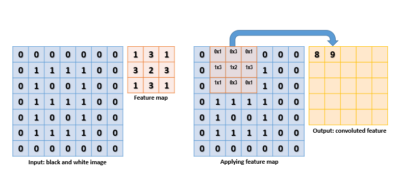
For example, for a [28 x 28] image and a 16 elements-deep feature map, the resulting hidden layer would be a tensor of dimension [28 x 28 x 16]. It is common to drop the outer pixels for which the filter would fall outside the image bounds; in that case, the resulting tensor dimensions will be reduced accordingly.

Activation Function Layer

A non-linear activation function is then applied to each unit output element of the convolutional layer. One of the most commonly used functions is the Rectified Linear Unit, or ReLU, which is simply max(0,x). Its practical advantage over a sigmoid function is that it does not suffer from the vanishing gradient problem, and therefore learning can be more efficient.

Max-Pooling Layer

"Max Pooling" is an operation placed after the activation function that aims at reducing dimensionality. It divides the input into a set of non-overlapping regions, where for each region it outputs the maximum activation value (independently for each depth slice). By reducing each region into a single point, the image dimension is reduced. What this achieves is two-fold: (1) it reduces the number of parameters and thus helps controlling overfitting; and (2) it selects the salient activation values regardless of their location in the region, which helps training models that are more resilient to things like rotation / translation. Here is an example (from Wikipedia) of max pooling with a window size of [2 x 2] (which would reduce a hidden layer of [28 x 28 x 16] to [14 x 14 x 16]):

Dense Layer

Finally, after cascading several convolutional, activation function, and MaxPooling layers, a CNN will have one or more fully connected, or dense, layers. Every unit in a dense layer has connections to all activations of the previous layer, similar to regular neural networks.

Softmax Layer

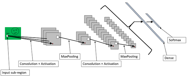
Finally, the softmax layer for classification. We know the softmax from the first part of the tutorial. The output is a probability distribution over the possible classes. Below is a chart of a CNN with two alternating convolution / activation and MaxPooling layers, one dense layer, and one softmax layer.

The Network Definition 2

Our CNN will have a bit more of a complex definition than our previous networks. Starting from the features, you will notice that we define each sample as a 28 x 28 matrix rather than a vector. This is because a CNN exploits local correlations in the image. Thus, we need to preserve this information. Second, in addition to the layer we saw in the previous network, we define a cascade of convolutional and max-pooling layers. We have two of each type. The core layer is ConvReLULayer which is defined as a function in Shared.bs. Here is what this macro looks like:

ConvReLULayer (inp, outMap, inWCount, kW, kH, hStride, vStride) = [
    convW = Parameter (outMap, inWCount, init="uniform", initValueScale=wScale)
    convB = ImageParameter (1, 1, outMap, init="fixedValue", value=bValue, imageLayout="$imageLayout$")
    conv = Convolution (convW, inp, kW, kH, outMap, hStride, vStride, zeroPadding=false, imageLayout="$imageLayout$")
    act = RectifiedLinear (conv + convB)
].act

(where wScale and bValue are expected to be declared outside).

The Convolution() built-in function that convolves (filters) the image with a kernel. If interested, please have a quick look here for the description of its parameters, before reading on.

We will also need the MaxPooling() operation. Please find its description here.

This allows us to put together the final network definition of our CNN that will learn to classify images of hand-written digits:

wScale = 10 ; bValue = 1 # in Shared.bs

imageW = 28
imageH = 28
labelDim = 10

features = ImageInput (imageW, imageH, 1, imageLayout="$imageLayout$")
featScaled = Constant(1/256) .* features)
labels = InputValue (labelDim)

# conv1
kW1 = 5
kH1 = 5
cMap1 = 16
hStride1 = 1
vStride1 = 1
# weight[cMap1, kW1 * kH1 * inputChannels]
# ConvReLULayer is defined in Shared.bs
conv1_act = ConvReLULayer (featScaled, cMap1, 25, kW1, kH1, hStride1, vStride1)

# pool1
pool1W = 2
pool1H = 2
pool1hStride = 2
pool1vStride = 2
pool1 = MaxPooling (conv1_act, pool1W, pool1H, pool1hStride, pool1vStride, imageLayout="$imageLayout$")

# conv2
kW2 = 5
kH2 = 5
cMap2 = 32
hStride2 = 1
vStride2 = 1
# weight[cMap2, kW2 * kH2 * cMap1]
# ConvReLULayer is defined in Shared.bs
conv2_act = ConvReLULayer (pool1, cMap2, 400, kW2, kH2, hStride2, vStride2, 10, 1)

# pool2
pool2W = 2
pool2H = 2
pool2hStride = 2
pool2vStride = 2
pool2 = MaxPooling (conv2_act, pool2W, pool2H, pool2hStride, pool2vStride, imageLayout="$imageLayout$")

h1Dim = 128
# DNNSigmoidLayer and DNNLayer are defined in Macros.ndl
h1 = DNNSigmoidLayer (512, h1Dim, pool2, 1)
ol = DNNLayer (h1Dim, labelDim, h1, 1)

ce = CrossEntropyWithSoftmax (labels, ol)
errs = ErrorPrediction (labels, ol)

# Special nodes
featureNodes    = (features)
labelNodes      = (labels)
criterionNodes  = (ce)
evaluationNodes = (errs)
outputNodes     = (ol)

Putting it all Together 2

Here are the configuration files you will need to run this example:

• The main configuration file incl. network definition
• The shared functions

Similar to the previous example, it runs using the following command:

cntk  configFile=../Config/02_Convolution_ndl_deprecated.cntk

The output folder will be created inside Image/MNIST/, and we get the test results on the console:

Final Results: Minibatch[1-625]: errs = 0.83% * 10000; ce = 0.02825477 * 10000

With an error of 0.83%, this model (unsurprisingly) greatly outperforms the previous one. It took only 2-3 minutes and 15 epochs to train on a single GPU. It is worth mentioning that with a GPU the results can vary slightly from run to run due to some non-deterministic CUDA functions. Let us compare the loss per epoch for the three models, softmax regression, one hidden layer network and CNN. As expected, loss for the CNN drops at a faster rate and reaches lower level than the loss of the other two models.

Now let's check out a technique that helps us to reduce the training time without significantly compromising the predictive performance of the model.

Improving Training: CNN with Batch Normalization

In this section we will add to our network a widely used technique called Batch Normalization. It helps to make training much more efficient. We will give a brief introduction before demonstrating how to add it to our CNN.

Batch Normalization in a Nutshell

One problem with training deep neural networks is that the distribution of each layer's inputs changes during training because the parameters of the previous layers change. This causes the training to slow down, as upper layers constantly have to adapt themselves to the changed ranges. One common technique to address the problem is called Batch Normalization (BN). BN consists of normalizing layer inputs w.r.t. their zero-mean/unit-variance, and to do so for each training minibatch. BN makes it possible to use much higher learning rates and allows us to be less careful about initialization. For more details, please refer to the paper here, and to the description of the BatchNormalization operation.

Disclaimer: Training with Batch Normalization is currently only supported on GPU (but models can be evaluated using the CPU).

The Network Definition 3

We start from the CNN we just built and add a batch normalization node to each layer's macro. Also, we change the sigmoid layer to a ReLU layer as it gives a slight bump to the model's accuracy.

imageW = 28
imageH = 28
labelDim = 10

features = ImageInput (imageW, imageH, 1, imageLayout="$imageLayout$")
featScaled = Constant(1/256) .* features)
labels = InputValue (labelDim)

scValue = 1
expAvg = 1

# conv1
kW1 = 5
kH1 = 5
cMap1 = 16
hStride1 = 1
vStride1 = 1
# weight[cMap1, kW1 * kH1 * inputChannels]
# ConvBNReLULayer is defined in Macros.ndl
conv1 = ConvBNReLULayer (featScaled, cMap1, 25, kW1, kH1, hStride1, vStride1, scValue, expAvg)

# pool1
pool1W = 2
pool1H = 2
pool1hStride = 2
pool1vStride = 2
pool1 = MaxPooling (conv1, pool1W, pool1H, pool1hStride, pool1vStride, imageLayout="$imageLayout$")

# conv2
kW2 = 5
kH2 = 5
cMap2 = 32
hStride2 = 1
vStride2 = 1
# weight[cMap2, kW2 * kH2 * cMap1]
conv2 = ConvBNReLULayer (pool1, cMap2, 400, kW2, kH2, hStride2, vStride2, scValue, expAvg)

# pool2
pool2W = 2
pool2H = 2
pool2hStride = 2
pool2vStride = 2
pool2 = MaxPooling (conv2, pool2W, pool2H, pool2hStride, pool2vStride, imageLayout="$imageLayout$")

h1Dim = 128
# DnnBNReLULayer is defined in Macros.ndl
h1 = DnnBNReLULayer (1568, h1Dim, pool2, scValue, expAvg)
ol = DNNLayer (h1Dim, labelDim, h1, 1)

ce = CrossEntropyWithSoftmax (labels, ol)
errs = ErrorPrediction (labels, ol)

# Special Nodes
featureNodes    = (features)
labelNodes      = (labels)
criterionNodes  = (ce)
evaluationNodes = (errs)
outputNodes     = (ol)

Putting it all Together 3

Here are the configuration files you need to run this example:

• The main configuration file
• The shared functions

Similar to the previous example, it runs using the following command:

cntk  configFile=../Config/03_ConvBatchNorm_ndl_deprecated.cntk

The output folder will be created inside Image/MNIST/, and we get the test results on the console:

Final Results: Minibatch[1-313]: errs = 0.96% * 10000; ce = 0.029642786 * 10000

With Batch Normalization the network achieves a tiny 0.96% error rate after training for just 2 epochs (and less than 30 seconds)!