Previous

Next

Exercise - Upload Data and Create Scatterplot

Completed

Jupyter notebooks are composed of cells. Each cell is assigned one of three types:

• Markdown for entering text in markdown format
• Code for entering code that runs interactively
• Raw NBConvert for entering data inline

Code entered into code cells is executed by a kernel, which provides an isolated environment for the notebook to run in. The popular IPython kernel supports code written in Python, but dozens of other kernels are available supporting other languages. Azure Notebooks support Python, R, and F# out of the box. They also support the installation of the many packages and libraries that are commonly used in research.

The notebook editor currently shows an empty cell. In this exercise, you will add content to that cell and add other cells to import Python packages such as NumPy, load a pair of NASA data files containing climate data, and create a scatter plot from the data.

1. In the first cell, set the cell type to Markdown and enter the "Azure Notebook Climate Change Analysis" into the cell itself:

   

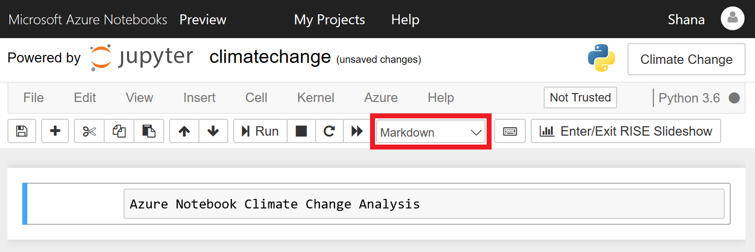
   Defining a markdown cell

2. Click the + button in the toolbar to add a new cell. Make sure the cell type is Code, and then enter the following Python code into the cell:

   import matplotlib.pyplot as plt
   import numpy as np
   from sklearn.linear_model import LinearRegression
   import seaborn as sns; sns.set()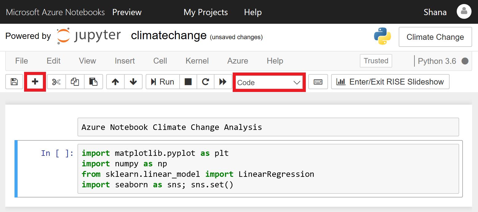
   

   

   Adding a code cell

3. Now click the Run button to run the code cell and import the packages specified in the import statements. Ignore any warnings that are displayed as the environment is prepared for the first time.

   You can remove the warnings by selecting the code cell and running it again.

   

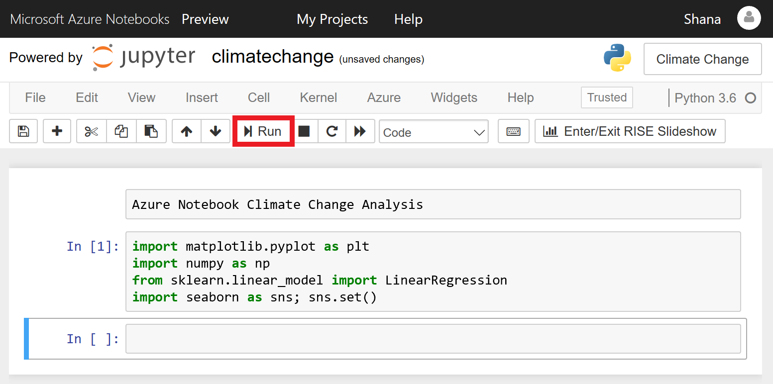
   Running a code cell

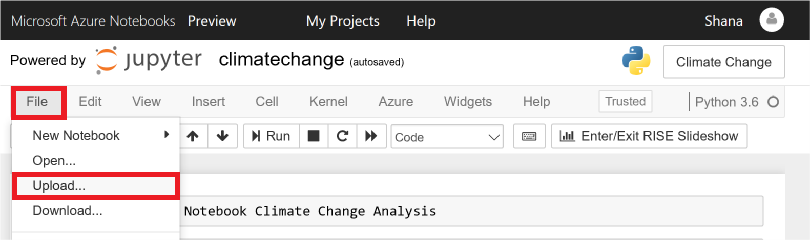
4. Click File in the menu at the top of the page, and select Upload from the drop-down menu. Then upload the files named 5-year-mean-1951-1980.csv and 5-year-mean-1882-2014.csv.

   

   Uploading data to the notebook

5. Select /project as your Destination Folder to ensure your files persist. Click Start Upload to upload the files, and OK once they successfully upload.

   

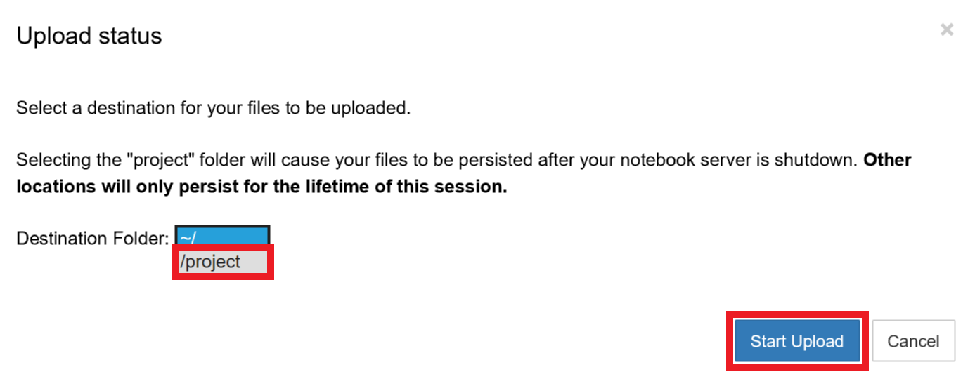
   Selecting destination folder for data

6. Place the cursor in the empty cell at the bottom of the notebook. Enter "Import data" as the text and change the cell type to Markdown.

7. Now add a Code cell and paste in the following code.

   yearsBase, meanBase = np.loadtxt('5-year-mean-1951-1980.csv', delimiter=',', usecols=(0, 1), unpack=True)
   years, mean = np.loadtxt('5-year-mean-1882-2014.csv', delimiter=',', usecols=(0, 1), unpack=True)
   

8. Click the Run button to run the cell and use NumPy's loadtxt function to load the data that you uploaded. The data is now in memory and can be used by the application.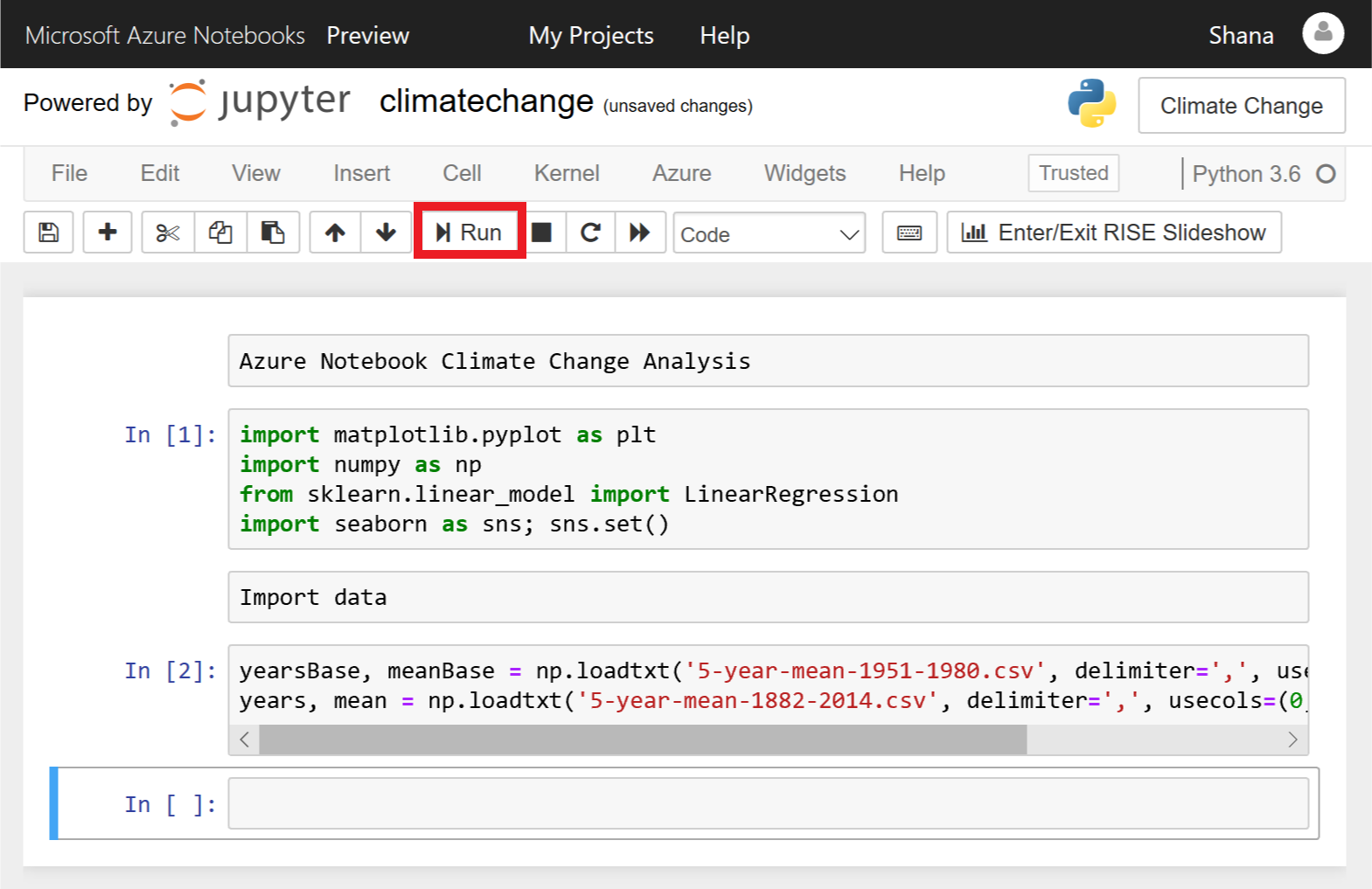

   

   Loading the data

9. Place the cursor in the empty cell at the bottom of the notebook. Change the cell type to Markdown and enter "Create a scatter plot" as the text.

10. Add a Code cell and paste in the following code, which uses Matplotlib to create a scatter plot.

    plt.scatter(yearsBase, meanBase)
    plt.title('scatter plot of mean temp difference vs year')
    plt.xlabel('years', fontsize=12)
    plt.ylabel('mean temp difference', fontsize=12)
    plt.show()
    

11. Click Run to run the cell and create a scatter plot.

    

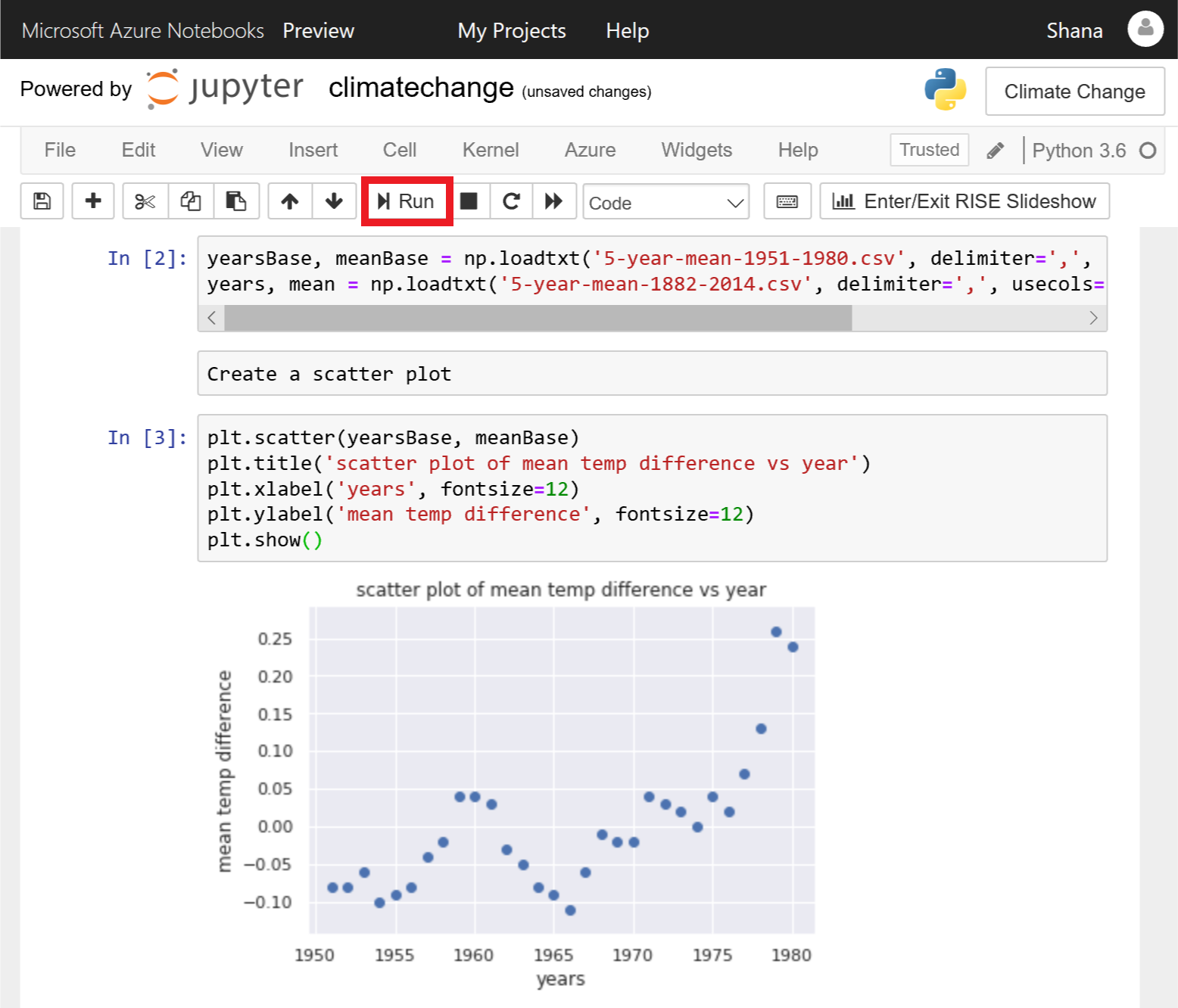
    Scatter plot produced by Matplotlib

The data set you loaded uses a 30-year mean between 1951 and 1980 to calculate a base temperature for that period, and then uses 5-year mean temperatures to calculate the difference between the 5-year mean and the 30-year mean for each year. The scatter plot shows the annual temperature differences.

Continue