Configure order promising
Order promising helps you reliably promise delivery dates to your customers and gives you flexibility so that you can meet those dates.
Order promising calculates the earliest ship and receipt dates and is based on the delivery date control method and transport days.
Based on the delivery date control type on the sales order line, Supply Chain Management calculates the earliest delivery date and populates the Requested ship date and the Requested receipt date. The Requested ship date is the earliest date that the company is able to dispatch the product's full line quantity from the warehouse that is specified on the line. The Requested receipt date is the earliest date that the product's full line quantity can be expected to be delivered to the customer's address.
The five delivery date control types are shown in the following image.
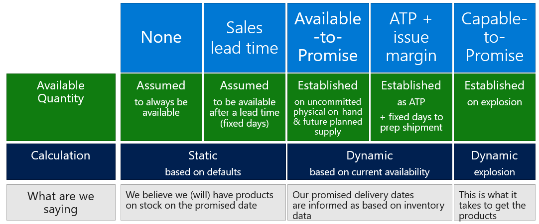
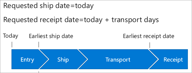
None
The following image shows the impact of order promising if the delivery date control is set to None. Order promising assumes that stock is always available and order shipment can be promised on the day that the order is taken.
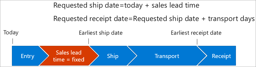
Sales lead time
The following image shows the impact of order promising if the delivery date control is set to Sales lead time. Sales lead time is the time between creation of the sales order and shipment of the items. The delivery date calculation is based on a default number of days and does not consider stock availability, known demand, or planned supply. You can define the lead time for a site. If no site-specific lead time is defined, the default setting for the item is used.
Order promising assumes that stock is available beyond the lead time and order shipment can be promised regardless of the actual availability.
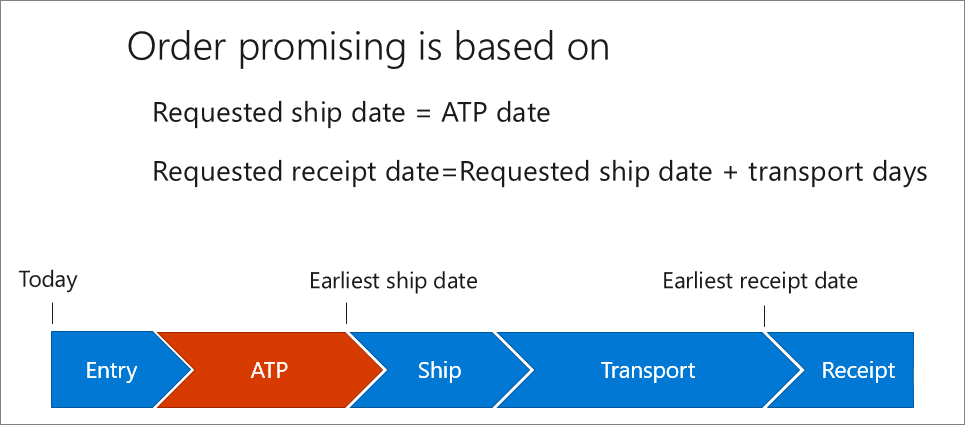
Available-to-promise (ATP)
ATP is the quantity of an item that is available and can be promised to a customer on a specific date. The ATP calculation includes uncommitted inventory, lead times, planned receipts, and issues.
ATP has the following features:
Delivery promises are based on real-time data.
Eliminates or reduces reservations as it considers sales order that are already entered (promised and unfulfilled).
Can be fine-tuned with margin time.
Considers business's working calendars as well as carriers' and customers' calendars.
Requires high delivery performance from suppliers.
Does not require a planning run and uses already existing supply.
Good fit for distribution industry and make-to-stock manufacturers.
Supports intercompany trade.
The following image shows the calculation of ATP. It checks uncommitted stock, supply, and committed demand.
ATP + issue margin
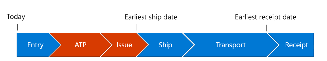
The earliest ship date is equal to the ATP date plus the issue margin for the item. The issue margin is the time that is required to prepare the items for shipment.
The following image shows the calculation of the ATP + issue margin. It checks uncommitted stock, supply, committed demand, and a fixed margin in days.
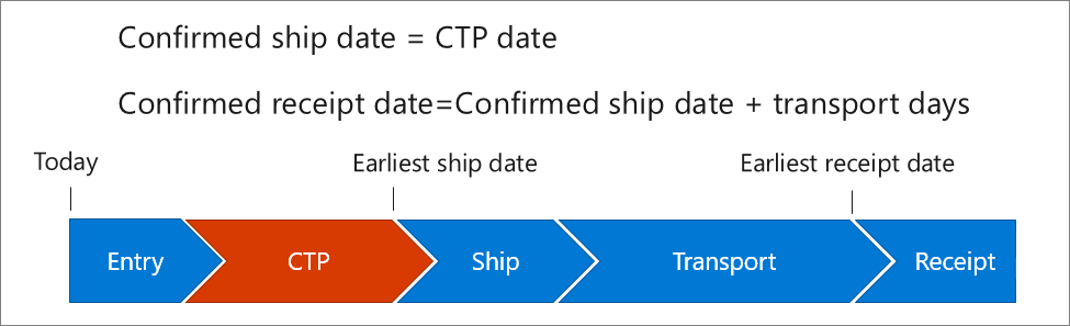
Capable-to-promise (CTP)
CTP is when order promising is based on a dynamic plan (sales order line explosion), checking availability and lead time components in the BOM and process time in the routes of the finished product.
Delivery alternatives
Sales order takers can use the Delivery alternatives page to discover alternative order fulfillment options.
The Delivery alternatives page layout gives an overview of all alternative options. It also lets order takers look beyond the current company for fulfillment opportunities. On this page, order takers can view both intercompany opportunities and opportunities from external vendors. By sorting the options by delivery date, sales order takers can view an intelligent list of delivery alternatives. In addition, parameters help them better manage the suggested deliveries. Because transport time can affect delivery dates, sales order takers can explore the various transportation choices that carriers offer.
Consider the following delivery alternatives:
Program-calculated recommendations for the earliest delivery date based on:
Availability across sites
Availability for variants
Partial quantity
Alternative transportation options
Sourcing from external vendor or through intercompany, cross-docking, or as direct delivery
Insights into existing demand and supply to potentially reallocate and expedite
Support for all delivery date control methods
Delivery control defaults
On the Accounts receivable parameters page, you can set up defaults for delivery control.

You can also set up the order promising of a product by going to Product information management > Products > Released products page.
ATP time fence
Calculate ATP by using the ATP time fence period (in days) if you selected the ATP calculation method in the Delivery date control field.
ATP backward demand time fence
Enter the number of days backward from today that past due demand (that is, inventory issues) will be considered when you are calculating the earliest available delivery dates for inventory. For example, if you enter 0, no past due demand will be considered. If you enter 1, yesterday's demand will be considered.
ATP backward supply time fence
Enter the number of days backward from today that past due supply (that is, inventory receipts) will be considered when you are calculating the earliest available delivery dates for inventory. For example, if you enter 0, no past due supply will be considered. If you enter 1, yesterday's supply will be considered.
ATP delayed demand offset time
The number of days into the future from today when past due demand on inventory issues will be considered as having its delivery date. For example, if you enter 0, items with a past due delivery date will be considered as delivered today. If you enter 1, items with a past due delivery date will be considered as delivered tomorrow.
ATP delayed supply offset time
The number of days into the future from today when items on past due inventory receipts will be considered as received. For example, if you enter 0, the item will be considered as received today. If you enter 1, the item will be considered as received tomorrow.
ATP incl. planned orders
Include planned orders in ATP calculations if you selected the ATP calculation method in the Delivery date control field.
ATP calculations
The ATP quantity is calculated by using the "cumulative ATP with look-ahead" method. The main advantage of this ATP calculation method is that it can handle cases where the sum of issues among receipts is more than the latest receipt (for example, when a quantity from an earlier receipt must be used to meet a requirement).
The "cumulative ATP with look-ahead" calculation method includes all issues until the cumulative quantity to receive exceeds the cumulative quantity to issue. Therefore, this ATP calculation method evaluates whether some of the quantity from an earlier period can be used in a later period.
The ATP quantity is the uncommitted inventory balance in the first period. Typically, it's calculated for each period in which a receipt is scheduled. The program calculates the ATP period in days and calculates the current date as the first date for the ATP quantity. In the first period, ATP includes on-hand inventory minus customer orders that are due and overdue.
ATP is calculated by using the following formula:
ATP = ATP for the previous period + Receipts for the current period - Issues for the current period - Net issue quantity for each future period until the period when the sum of receipts for all future periods, up to and including the future period, exceeds the sum of issues up to and including the future period.
When no more issues or receipts are left to consider, the ATP quantity for the following dates is the same as the latest calculated ATP quantity.
If not all the dimensions that are used for an item are given when the ATP check is completed, they can still be specified on the issue and receipts. In this case, in the ATP calculation, the receipts and issues must be aggregated to the existing dimensions to reduce the number of receipt and issue lines that are used in the ATP calculation.
The ATP quantity that is shown is always greater than or equal to 0 (zero). If the calculation returns a negative ATP quantity (for example, if the quantity that was previously promised exceeds the available quantity), the program automatically sets the quantity to 0.
The ATP backward demand time fence field controls how far back in time to look for delayed demand orders or inventory issues.
The ATP backward supply time fence field controls how far back in time to look for delayed supply orders or inventory receipts. For example, if orders that are delayed by only seven days should be considered in the ATP calculation, both fields should be set to 7.
The ATP delayed demand offset time and ATP delayed supply offset time fields control when the delayed demand or supply will be considered in the ATP calculation. For example, if the delayed supply and demand should be considered in the ATP calculation the day after tomorrow, both fields should be set to 2. A value of 2 means that the quantity of an item on a delayed purchase order that should be considered in the ATP calculation will be shown as available two days after the current date.