Exercise - Use machine learning and standard deviation to create fictional game data - Training

5 minutes

We've run into a problem. We can't get real-time game data from the Tune Squad playing. There's no way for us to watch a game of 15 Tune Squad characters playing basketball and test out our model in an actual app.

But, we can use the trick we learned about testing our model to create a new dataset that will simulate a game!

The web app that we'll build in the upcoming units will help us decide which player to give a water break to every 12 minutes of a standard 48-minute game. So, we should create a CSV file that will contain randomized player data over four iterations: 0 minutes (the start of the game), 12 minutes, 24 minutes, and 36 minutes:

# Initialize four empty DataFrames, one for each 12-minute period.
number_of_iterations = 4
df_list = [pd.DataFrame(columns=game_stat_cols, index=list(ts_df['player_name'])) for i in range(number_of_iterations)]

# For each period, generate randomized player data and predict the PER.
# Use the model fitted earlier.
for df in df_list:
    for stat in game_stat_cols:
        df[stat] = list(ts_df[stat] + randn(len(ts_df)) * stdev_s[stat])
    df['PER'] = lin_reg.predict(df)

# Concatenate the DataFrames and make the players' names the index.
game_df = pd.concat(df_list)
game_df.rename_axis('player_name', inplace=True)

# Create another index for the period in question.
minutes = [(x // len(ts_df)) * 12 for x in range(len(game_df))]
game_df['minutes'] = minutes
game_df.set_index('minutes', append=True, inplace=True)
game_df = game_df.swaplevel()

game_df

Here's the output:

minutes	player_name	TS%	AST	TO	USG	ORR	DRR	REBR	PER
0	Sylvester	0.617897	31.998307	16.008589	39.097789	6.413572	15.286788	12.792845	31.761414
	Marvin the Martian	0.605018	33.807167	13.666316	34.011445	6.441147	18.954713	15.582038	31.065373
	Road Runner	0.606381	29.732153	15.027962	38.444237	4.532569	27.268949	10.968630	21.550397
	Foghorn Leghorn	0.606442	31.879217	15.467578	36.674624	6.019145	20.964740	14.774713	29.283807
	Bugs Bunny	0.636505	35.193108	15.708836	37.962839	6.116200	23.132887	15.677267	31.850749
...	...	...	...	...	...	...	...	...	...
36	Granny	0.608159	26.021605	14.814805	31.721274	6.422251	22.213857	16.454224	27.644534
	Wile E. Coyote	0.601998	29.851305	14.137783	32.102558	5.819653	25.550118	15.818051	25.497379
	Tweety	0.607711	25.210393	12.609053	34.014773	6.628928	27.041059	11.643892	20.439595
	Penelope	0.613901	25.007772	14.394944	28.324923	7.564207	23.184055	9.919301	16.124275
	Daffy Duck	0.634848	31.911011	14.694308	33.226023	6.308140	18.023737	16.305183	33.155391

60 rows × eight columns

The final DataFrame looks complete. We can save it as a CSV file, so we can use it in our web app. When saving this DataFrame as a CSV file, we'll want to keep the indices, because we made them the player's names.

# Export the finished DataFrame to CSV.
game_df.to_csv('game_stats.csv')

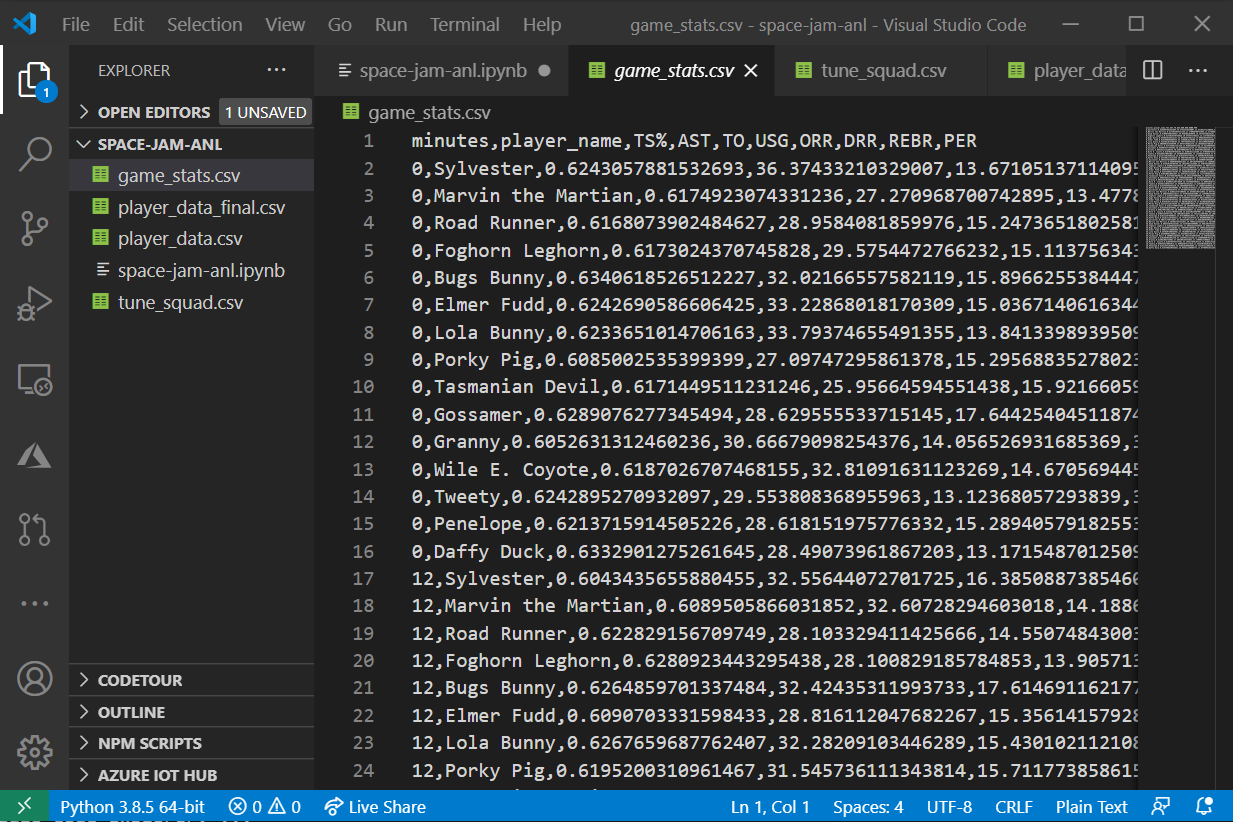
A new CSV file should appear in your Visual Studio Code folder:

Screenshot that shows the game stats C S V file in Visual Studio Code Explorer.

Continue

Exercise - Use machine learning and standard deviation to create fictional game data

Feedback