Overview of forecasting methods in AutoML
This article focuses on the methods that AutoML uses to prepare time series data and build forecasting models. Instructions and examples for training forecasting models in AutoML can be found in our set up AutoML for time series forecasting article.
AutoML uses several methods to forecast time series values. These methods can be roughly assigned to two categories:
- Time series models that use historical values of the target quantity to make predictions into the future.
- Regression, or explanatory, models that use predictor variables to forecast values of the target.
As an example, consider the problem of forecasting daily demand for a particular brand of orange juice from a grocery store. Let $y_t$ represent the demand for this brand on day $t$. A time series model predicts demand at $t+1$ using some function of historical demand,
$y_{t+1} = f(y_t, y_{t-1}, \ldots, y_{t-s})$.
The function $f$ often has parameters that we tune using observed demand from the past. The amount of history that $f$ uses to make predictions, $s$, can also be considered a parameter of the model.
The time series model in the orange juice demand example may not be accurate enough since it only uses information about past demand. There are many other factors that likely influence future demand such as price, day of the week, and whether it's a holiday or not. Consider a regression model that uses these predictor variables,
$y = g(\text{price}, \text{day of week}, \text{holiday})$.
Again, $g$ generally has a set of parameters, including those governing regularization, that AutoML tunes using past values of the demand and the predictors. We omit $t$ from the expression to emphasize that the regression model uses correlational patterns between contemporaneously defined variables to make predictions. That is, to predict $y_{t+1}$ from $g$, we must know which day of the week $t+1$ falls on, whether it's a holiday, and the orange juice price on day $t+1$. The first two pieces of information are always easily found by consulting a calendar. A retail price is usually set in advance, so the price of orange juice is likely also known one day ahead. However, the price may not be known 10 days into the future! It's important to understand that the utility of this regression is limited by how far into the future we need forecasts, also called the forecast horizon, and to what degree we know the future values of the predictors.
Important
AutoML's forecasting regression models assume that all features provided by the user are known into the future, at least up to the forecast horizon.
AutoML's forecasting regression models can also be augmented to use historical values of the target and predictors. The result is a hybrid model with characteristics of a time series model and a pure regression model. Historical quantities are additional predictor variables in the regression and we refer to them as lagged quantities. The order of the lag refers to how far back the value is known. For example, the current value of an order-two lag of the target for our orange juice demand example is the observed juice demand from two days ago.
Another notable difference between the time series models and the regression models is in the way they generate forecasts. Time series models are generally defined by recursion relations and produce forecasts one-at-a-time. To forecast many periods into the future, they iterate up-to the forecast horizon, feeding previous forecasts back into the model to generate the next one-period-ahead forecast as needed. In contrast, the regression models are so-called direct forecasters that generate all forecasts up to the horizon in one go. Direct forecasters can be preferable to recursive ones because recursive models compound prediction error when they feed previous forecasts back into the model. When lag features are included, AutoML makes some important modifications to the training data so that the regression models can function as direct forecasters. See the lag features article for more details.
Forecasting models in AutoML
The following table lists the forecasting models implemented in AutoML and what category they belong to:
| Time Series Models | Regression Models |
|---|---|
| Naive, Seasonal Naive, Average, Seasonal Average, ARIMA(X), Exponential Smoothing | Linear SGD, LARS LASSO, Elastic Net, Prophet, K Nearest Neighbors, Decision Tree, Random Forest, Extremely Randomized Trees, Gradient Boosted Trees, LightGBM, XGBoost, TCNForecaster |
The models in each category are listed roughly in order of the complexity of patterns they're able to incorporate, also known as the model capacity. A Naive model, which simply forecasts the last observed value, has low capacity while the Temporal Convolutional Network (TCNForecaster), a deep neural network with potentially millions of tunable parameters, has high capacity.
Importantly, AutoML also includes ensemble models that create weighted combinations of the best performing models to further improve accuracy. For forecasting, we use a soft voting ensemble where composition and weights are found via the Caruana Ensemble Selection Algorithm.
Note
There are two important caveats for forecast model ensembles:
- The TCN cannot currently be included in ensembles.
- AutoML by default disables another ensemble method, the stack ensemble, which is included with default regression and classification tasks in AutoML. The stack ensemble fits a meta-model on the best model forecasts to find ensemble weights. We've found in internal benchmarking that this strategy has an increased tendency to over fit time series data. This can result in poor generalization, so the stack ensemble is disabled by default. However, it can be enabled if desired in the AutoML configuration.
How AutoML uses your data
AutoML accepts time series data in tabular, "wide" format; that is, each variable must have its own corresponding column. AutoML requires one of the columns to be the time axis for the forecasting problem. This column must be parsable into a datetime type. The simplest time series data set consists of a time column and a numeric target column. The target is the variable one intends to predict into the future. The following is an example of the format in this simple case:
| timestamp | quantity |
|---|---|
| 2012-01-01 | 100 |
| 2012-01-02 | 97 |
| 2012-01-03 | 106 |
| ... | ... |
| 2013-12-31 | 347 |
In more complex cases, the data may contain other columns aligned with the time index.
| timestamp | SKU | price | advertised | quantity |
|---|---|---|---|---|
| 2012-01-01 | JUICE1 | 3.5 | 0 | 100 |
| 2012-01-01 | BREAD3 | 5.76 | 0 | 47 |
| 2012-01-02 | JUICE1 | 3.5 | 0 | 97 |
| 2012-01-02 | BREAD3 | 5.5 | 1 | 68 |
| ... | ... | ... | ... | ... |
| 2013-12-31 | JUICE1 | 3.75 | 0 | 347 |
| 2013-12-31 | BREAD3 | 5.7 | 0 | 94 |
In this example, there's a SKU, a retail price, and a flag indicating whether an item was advertised in addition to the timestamp and target quantity. There are evidently two series in this dataset - one for the JUICE1 SKU and one for the BREAD3 SKU; the SKU column is a time series ID column since grouping by it gives two groups containing a single series each. Before sweeping over models, AutoML does basic validation of the input configuration and data and adds engineered features.
Data length requirements
To train a forecasting model, you must have a sufficient amount of historical data. This threshold quantity varies with the training configuration. If you've provided validation data, the minimum number of training observations required per time series is given by,
$T_{\text{user validation}} = H + \text{max}(l_{\text{max}}, s_{\text{window}}) + 1$,
where $H$ is the forecast horizon, $l_{\text{max}}$ is the maximum lag order, and $s_{\text{window}}$ is the window size for rolling aggregation features. If you're using cross-validation, the minimum number of observations is,
$T_{\text{CV}} = 2H + (n_{\text{CV}} - 1) n_{\text{step}} + \text{max}(l_{\text{max}}, s_{\text{window}}) + 1$,
where $n_{\text{CV}}$ is the number of cross-validation folds and $n_{\text{step}}$ is the CV step size, or offset between CV folds. The basic logic behind these formulas is that you should always have at least a horizon of training observations for each time series, including some padding for lags and cross-validation splits. See forecasting model selection for more details on cross-validation for forecasting.
Missing data handling
AutoML's time series models require regularly spaced observations in time. Regularly spaced, here, includes cases like monthly or yearly observations where the number of days between observations may vary. Prior to modeling, AutoML must ensure there are no missing series values and that the observations are regular. Hence, there are two missing data cases:
- A value is missing for some cell in the tabular data
- A row is missing which corresponds with an expected observation given the time series frequency
In the first case, AutoML imputes missing values using common, configurable techniques.
An example of a missing, expected row is shown in the following table:
| timestamp | quantity |
|---|---|
| 2012-01-01 | 100 |
| 2012-01-03 | 106 |
| 2012-01-04 | 103 |
| ... | ... |
| 2013-12-31 | 347 |
This series ostensibly has a daily frequency, but there's no observation for Jan. 2, 2012. In this case, AutoML will attempt to fill in the data by adding a new row for Jan. 2, 2012. The new value for the quantity column, and any other columns in the data, will then be imputed like other missing values. Clearly, AutoML must know the series frequency in order to fill in observation gaps like this. AutoML automatically detects this frequency, or, optionally, the user can provide it in the configuration.
The imputation method for filling missing values can be configured in the input. The default methods are listed in the following table:
| Column Type | Default Imputation Method |
|---|---|
| Target | Forward fill (last observation carried forward) |
| Numeric Feature | Median value |
Missing values for categorical features are handled during numerical encoding by including an additional category corresponding to a missing value. Imputation is implicit in this case.
Automated feature engineering
AutoML generally adds new columns to user data to increase modeling accuracy. Engineered feature can include the following:
| Feature Group | Default/Optional |
|---|---|
| Calendar features derived from the time index (for example, day of week) | Default |
| Categorical features derived from time series IDs | Default |
| Encoding categorical types to numeric type | Default |
| Indicator features for holidays associated with a given country or region | Optional |
| Lags of target quantity | Optional |
| Lags of feature columns | Optional |
| Rolling window aggregations (for example, rolling average) of target quantity | Optional |
| Seasonal decomposition (STL) | Optional |
You can configure featurization from the AutoML SDK via the ForecastingJob class or from the Azure Machine Learning studio web interface.
Non-stationary time series detection and handling
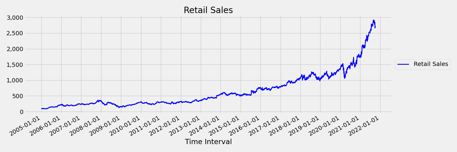
A time series where mean and variance change over time is called a non-stationary. For example, time series that exhibit stochastic trends are non-stationary by nature. To visualize this, the following image plots a series that is generally trending upward. Now, compute and compare the mean (average) values for the first and the second half of the series. Are they the same? Here, the mean of the series in the first half of the plot is significantly smaller than in the second half. The fact that the mean of the series depends on the time interval one is looking at, is an example of the time-varying moments. Here, the mean of a series is the first moment.
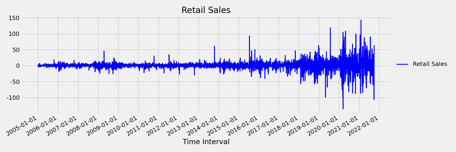
Next, let's examine the following image, which plots the original series in first differences, $\Delta y_{t} = y_t - y_{t-1}$. The mean of the series is roughly constant over the time range while the variance appears to vary. Thus, this is an example of a first order stationary times series.
AutoML regression models can't inherently deal with stochastic trends, or other well-known problems associated with non-stationary time series. As a result, out-of-sample forecast accuracy can be poor if such trends are present.
AutoML automatically analyzes time series dataset to determine stationarity. When non-stationary time series are detected, AutoML applies a differencing transform automatically to mitigate the impact of non-stationary behavior.
Model sweeping
After data has been prepared with missing data handling and feature engineering, AutoML sweeps over a set of models and hyper-parameters using a model recommendation service. The models are ranked based on validation or cross-validation metrics and then, optionally, the top models may be used in an ensemble model. The best model, or any of the trained models, can be inspected, downloaded, or deployed to produce forecasts as needed. See the model sweeping and selection article for more details.
Model grouping
When a dataset contains more than one time series, as in the given data example, there are multiple ways to model that data. For instance, we may simply group by the time series ID column(s) and train independent models for each series. A more general approach is to partition the data into groups that may each contain multiple, likely related series and train a model per group. By default, AutoML forecasting uses a mixed approach to model grouping. Time series models, plus ARIMAX and Prophet, assign one series to one group and other regression models assign all series to a single group. The following table summarizes the model groupings in two categories, one-to-one and many-to-one:
| Each Series in Own Group (1:1) | All Series in Single Group (N:1) |
|---|---|
| Naive, Seasonal Naive, Average, Seasonal Average, Exponential Smoothing, ARIMA, ARIMAX, Prophet | Linear SGD, LARS LASSO, Elastic Net, K Nearest Neighbors, Decision Tree, Random Forest, Extremely Randomized Trees, Gradient Boosted Trees, LightGBM, XGBoost, TCNForecaster |
More general model groupings are possible via AutoML's Many-Models solution; see our Many Models- Automated ML notebook.
Next steps
- Learn about deep learning models for forecasting in AutoML
- Learn more about model sweeping and selection for forecasting in AutoML.
- Learn about how AutoML creates features from the calendar.
- Learn about how AutoML creates lag features.
- Read answers to frequently asked questions about forecasting in AutoML.
Tilbakemeldinger
Kommer snart: Gjennom 2024 faser vi ut GitHub Issues som tilbakemeldingsmekanisme for innhold, og erstatter det med et nytt system for tilbakemeldinger. Hvis du vil ha mer informasjon, kan du se: https://aka.ms/ContentUserFeedback.
Send inn og vis tilbakemelding for