APPLIES TO:  Power BI Desktop
Power BI service
Power BI Desktop
Power BI service
With conditional formatting for tables and matrixes in Power BI, you can specify customized cell colors, including color gradients, based on field values. You can also represent cell values with data bars or KPI icons, or as active web links. You can apply conditional formatting to any text or data field, as long as you base the formatting on a field that has numeric, color name or hex code, or web URL values.
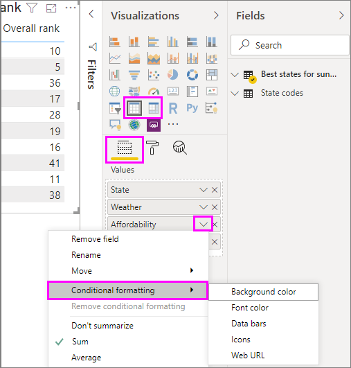
To apply conditional formatting, select a Table or Matrix visualization in Power BI Desktop or the Power BI service. In the Visualizations pane, right-click or select the down-arrow next to the field in the Values well that you want to format. Select Conditional formatting, and then select the type of formatting to apply.
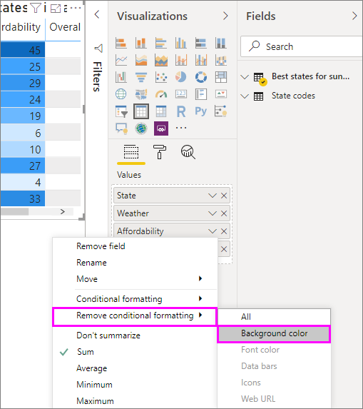
To remove conditional formatting from a visualization, select Remove conditional formatting from the field's drop-down menu, and then select the type of formatting to remove.
Note
Conditional formatting overrides any custom background or font color you apply to the conditionally formatted cell.
The following sections describe each conditional formatting option. You can combine more than one option in a single table column.
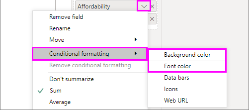
To format cell background or font color, select Conditional formatting for a field, and then select either Background color or Font color from the drop-down menu.
The Background color or Font color dialog box opens, with the name of the field you're formatting in the title. After selecting conditional formatting options, select OK.
The Background color and Font color options are the same, but affect the cell background color and font color, respectively. You can apply the same or different conditional formatting to a field's font color and background color. If you make a field's font and background the same color, the font blends into the background so the table column shows only the colors.
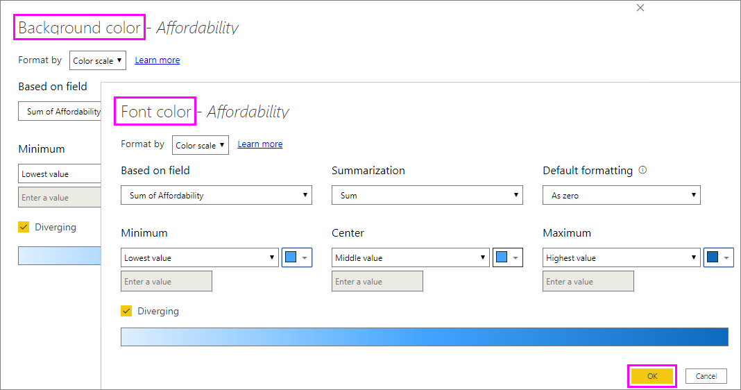
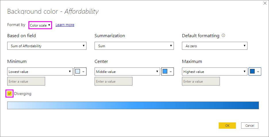
To format cell background or font color by color scale, in the Format style field of the Background color or Font color dialog box, select Gradient. Under What field should we based this on?, select the field to base the formatting on. You can base the formatting on the current field, or on any field in your model that has numerical or color data.
Under Summarization, specify the aggregation type you want to use for the selected field. Under Default formatting, select a formatting to apply to blank values.
Under Minimum and Maximum, choose whether to apply the color scheme based on the lowest and highest field values, or on custom values you enter. Select the drop-down and select the colors swatches you want to apply to the minimum and maximum values. Select the Add a middle color check box to also specify a Center value and color.
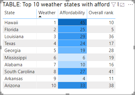
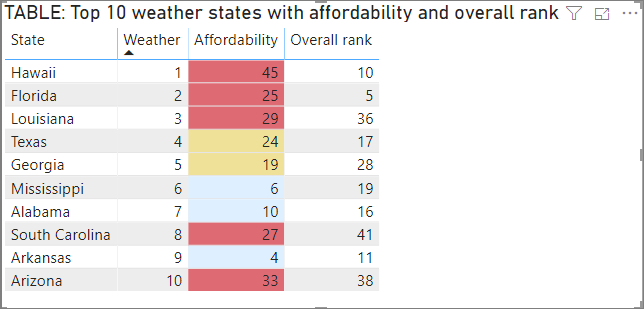
An example table with color scale background formatting on the Affordability column looks like this:
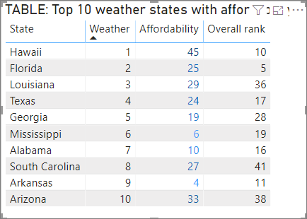
The example table with color scale font formatting on the Affordability column looks like this:
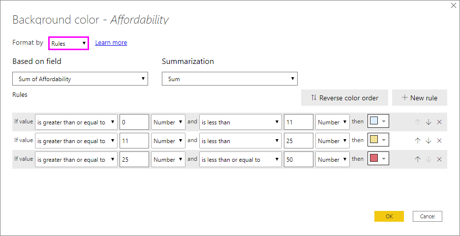
To format cell background or font color by rules, in the Format style field of the Background color or Font color dialog box, select Rules. Again, What field should we base this on? shows the field to base the formatting on, and Summarization shows the aggregation type for the field.
Under Rules, enter one or more value ranges, and set a color for each one. Each value range has an If value condition, an and value condition, and a color. Cell backgrounds or fonts in each value range are colored with the given color. The following example has three rules:
When you select Percent in this dropdown, you’re setting the rule boundaries as a percent of the overall range of values from minimum to maximum. So, for example, if the lowest data point was 100 and the highest was 400, the above rules would color any point less than 200 as green, anything from 200 to 300 as yellow, and anything above 300 as red.
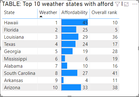
An example table with rules-based background color formatting based on Percent in the Affordability column looks like this:
Color by rules for percentages
If the field the formatting is based on contains percentages, write the numbers in the rules as decimals, which are the actual values; for example, ".25" instead of "25". Also, select Number instead of Percent for the number format. For example, "If value is greater than or equal to 0 Number and is less than .25 Number" returns values less than 25%.

In this example table with rules-based background color on the % revenue region column, 0 to 25% is red, 26% to 41% is yellow, and 42% and more is blue:

Note
If you use Percent instead of Number for fields containing percentages, you may get unexpected results. In the above example, in a range of percent values from 21.73% to 44.36%, 50% of that range is 33%. So use Number instead.
If you have a field or measure with color name or hex value data, you can use conditional formatting to automatically apply those colors to a column's background or font color. You can also use custom logic to apply colors to the font or background.
The field can use any color values listed in the CSS color spec at https://www.w3.org/TR/css-color-3/. These color values can include:
- 3, 6 or 8-digit hex codes, for example #3E4AFF. Make sure you include the # symbol at the start of the code.
- RGB or RGBA values, like RGBA(234, 234, 234, 0.5).
- HSL or HSLA values, like HSLA(123, 75%, 75%, 0.5).
- Color names, such as Green, SkyBlue, or PeachPuff.
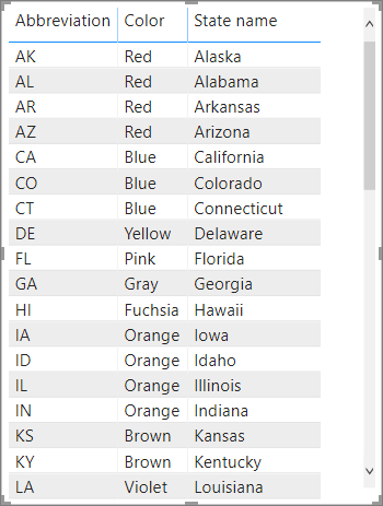
The following table has a color name associated with each state:
To format the Color column based on its field values, select Conditional formatting for the Color field, and then select Background color or Font color.
In the Background color or Font color dialog box, select Field value from the Format style drop-down field.

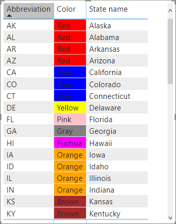
An example table with color field value-based Background color formatting on the Color field looks like this:
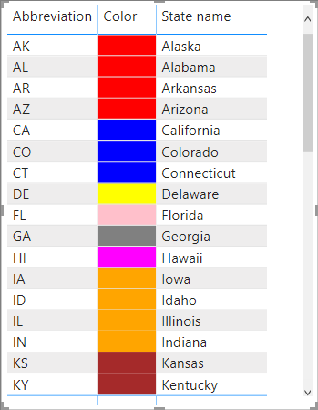
If you also use Field value to format the column's Font color, the result is a solid color in the Color column:
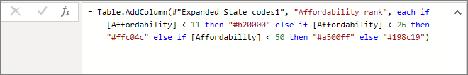
Color based on a calculation
You can create a calculation that outputs different values based on business logic conditions you select. Creating a formula is usually faster than creating multiple rules in the conditional formatting dialog.
For example, the following formula applies hex color values to a new Affordability rank column, based on existing Affordability column values:
To apply the colors, select Background color or Font color conditional formatting for the Affordability column, and base the formatting on the Field value of the Affordability rank column.
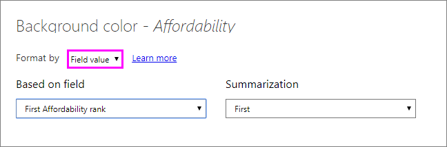
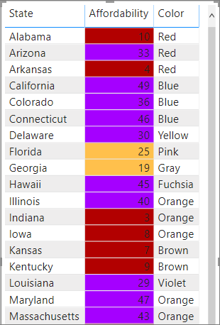
The example table with Affordability background color based on calculated Affordability rank looks like this:
You can create many more variations, just by using your imagination and some calculations.
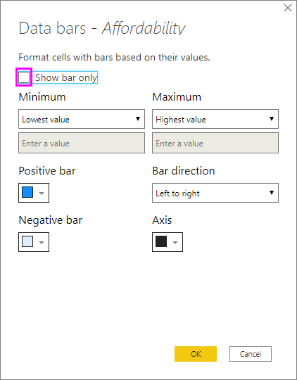
To show data bars based on cell values, select Conditional formatting for the Affordability field, and then select Data bars from the drop-down menu.
In the Data bars dialog, the Show bar only option is unchecked by default, so the table cells show both the bars and the actual values. To show the data bars only, select the Show bar only check box.
You can specify Minimum and Maximum values, data bar colors and direction, and axis color.
With data bars applied to the Affordability column, the example table looks like this:
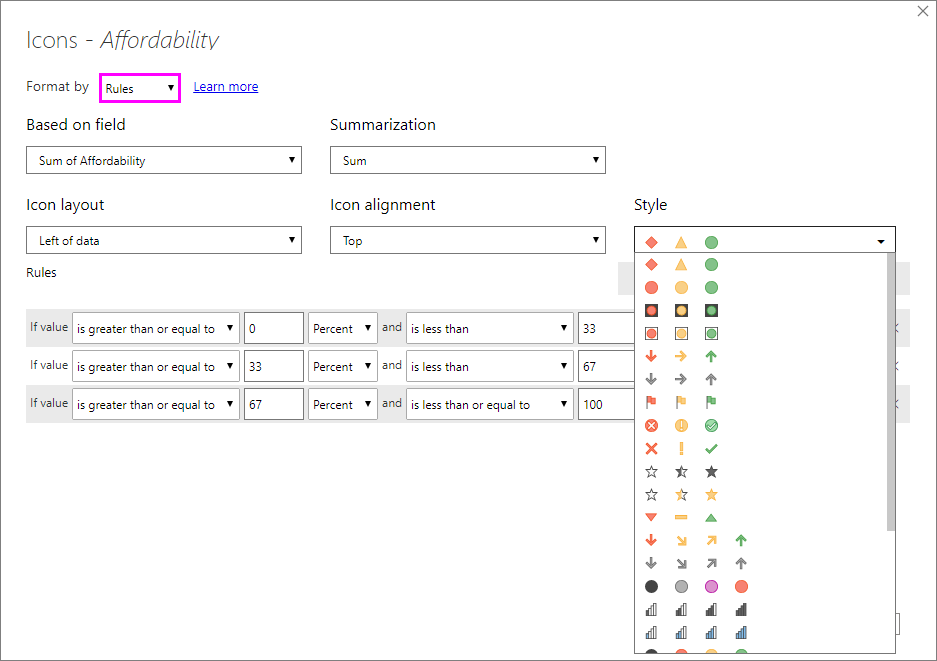
To show icons based on cell values, select Conditional formatting for the field, and then select Icons from the drop-down menu.
In the Icons dialog, under Format style, select either Rules or Field value.
To format by rules, select a What field should we base this on?, Summarization method, Icon layout, Icon alignment, icon Style, and one or more Rules. Under Rules, enter one or more rules with an If value condition and an and value condition, and select an icon to apply to each rule.
To format by field values, select a What field should we base this on?, Summarization method, Icon layout, and Icon alignment.
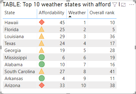
The following example adds icons based on three rules:
Select OK. With icons applied to the Affordability column by rules, the example table looks like this:
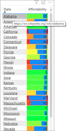
If you have a column or measure that contains website URLs, you can use conditional formatting to apply those URLs to fields as active links. For example, the following table has a Website column with website URLs for each state:

To display each state name as a live link to its website, select Conditional formatting for the State field, and then select Web URL. In the Web URL dialog box, under What field should we based this on?, select Website, and then select OK.
With Web URL formatting applied to the State field, each state name is an active link to its website. The following example table has Web URL formatting applied to the State column, and conditional Data bars applied to the Overall rank column.
See Add hyperlinks (URLs) to a table or matrix for more on formatting URLs in a table.
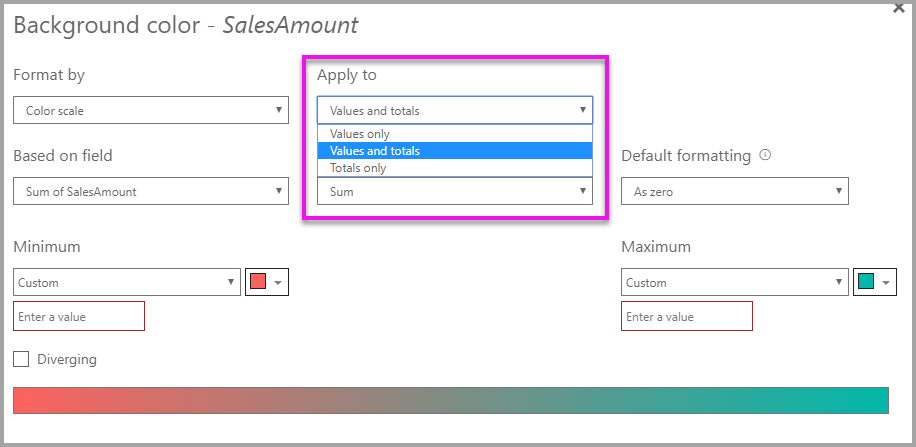
You can apply conditional formatting rules to totals and subtotals, for both table and matrix visuals.
You apply the conditional formatting rules by using the Apply to drop-down in conditional formatting, as shown in the following image.
You must manually set the thresholds and ranges for conditional formatting rules. For matrices, Values will refer to the lowest visible level of the matrix hierarchy.
Unlike in Excel, you can't color-code text values to display as a particular color, such as "Accepted"=blue, "Declined"=red, "None"=grey. You create measures related to these values and apply formatting based on those instead.
For example, StatusColor = SWITCH('Table'[Status], "Accepted", "blue", "Declined", "red", "None", "grey")
Then in the Background color dialog box, you format the Status field based on the values in the StatusColor field.

In the resulting table, the formatting is based on the value in the StatusColor field, which in turn is based on the text in the Status field.

Considerations and limitations
There are a few considerations to keep in mind when working with conditional table formatting:
- Any table that doesn't have a grouping is displayed as a single row that doesn't support conditional formatting.
- You can't apply gradient formatting with automatic maximum/minimum values, or rule-based formatting with percentage rules, if your data contains NaN values. NaN means "Not a number," most commonly caused by a divide by zero error. You can use the DIVIDE() DAX function to avoid these errors.
- Conditional formatting needs an aggregation or measure to be applied to the value. That's why you see 'First' or 'Last' in the Color by value example. If you're building your report against an Analysis Service multidimensional cube, you won't be able to use an attribute for conditional formatting unless the cube owner builds a measure that provides the value.
- When printing a report including data bars and background color, you must enable Background graphics in the print settings of the browser for the data bars and background colors to print properly.
For more information about color formatting, see Tips and tricks for color formatting in Power BI