Note
Access to this page requires authorization. You can try signing in or changing directories.
Access to this page requires authorization. You can try changing directories.
The Excel JavaScript Library provides APIs to apply conditional formatting to data ranges in your worksheets. This functionality makes large sets of data easy to visually parse. The formatting also dynamically updates based on changes within the range.
Note
This article covers conditional formatting in the context of Excel JavaScript add-ins. The following articles provide detailed information about the full conditional formatting capabilities within Excel.
The Range.conditionalFormats property is a collection of ConditionalFormat objects that apply to the range. The ConditionalFormat object contains several properties that define the format to be applied based on the ConditionalFormatType.
cellValuecolorScalecustomdataBariconSetpresettextComparisontopBottom
Note
Each of these formatting properties has a corresponding *OrNullObject variant. Learn more about that pattern in the *OrNullObject methods section.
Only one format type can be set for the ConditionalFormat object. This is determined by the type property, which is a ConditionalFormatType enum value. type is set when adding a conditional format to a range.
Conditional formats are added to a range by using conditionalFormats.add. Once added, the properties specific to the conditional format can be set. The following examples show the creation of different formatting types.
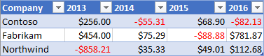
Cell value conditional formatting applies a user-defined format based on the results of one or two formulas in the ConditionalCellValueRule. The operator property is a ConditionalCellValueOperator defining how the resulting expressions relate to the formatting.
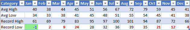
The following example shows red font coloring applied to any value in the range less than zero.
await Excel.run(async (context) => {
    const sheet = context.workbook.worksheets.getItem("Sample");
    const range = sheet.getRange("B21:E23");
    const conditionalFormat = range.conditionalFormats.add(
        Excel.ConditionalFormatType.cellValue
    );

    // Set the font of negative numbers to red.
    conditionalFormat.cellValue.format.font.color = "red";
    conditionalFormat.cellValue.rule = { formula1: "=0", operator: "LessThan" };

    await context.sync();
});
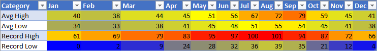
Color scale conditional formatting applies a color gradient across the data range. The criteria property on the ColorScaleConditionalFormat defines three ConditionalColorScaleCriterion: minimum, maximum, and, optionally, midpoint. Each of the criterion scale points have three properties:
color- The HTML color code for the endpoint.formula- A number or formula representing the endpoint. This will benulliftypeislowestValueorhighestValue.type- How the formula should be evaluated.highestValueandlowestValuerefer to values in the range being formatted.
The following example shows a range being colored blue to yellow to red. Note that minimum and maximum are the lowest and highest values respectively and use null formulas. midpoint is using the percentage type with a formula of "=50" so the yellowest cell is the mean value.
await Excel.run(async (context) => {
    const sheet = context.workbook.worksheets.getItem("Sample");
    const range = sheet.getRange("B2:M5");
    const conditionalFormat = range.conditionalFormats.add(
          Excel.ConditionalFormatType.colorScale
    );

    // Color the backgrounds of the cells from blue to yellow to red based on value.
    const criteria = {
          minimum: {
               formula: null,
               type: Excel.ConditionalFormatColorCriterionType.lowestValue,
               color: "blue"
          },
          midpoint: {
               formula: "50",
               type: Excel.ConditionalFormatColorCriterionType.percent,
               color: "yellow"
          },
          maximum: {
               formula: null,
               type: Excel.ConditionalFormatColorCriterionType.highestValue,
               color: "red"
          }
    };
    conditionalFormat.colorScale.criteria = criteria;

    await context.sync();
});
Custom conditional formatting applies a user-defined format to the cells based on a formula of arbitrary complexity. The ConditionalFormatRule object lets you define the formula in different notations:
formula- Standard notation.formulaLocal- Localized based on the user's language.formulaR1C1- R1C1-style notation.
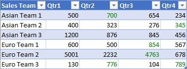
The following example colors the fonts green of cells with higher values than the cell to their left.
await Excel.run(async (context) => {
    const sheet = context.workbook.worksheets.getItem("Sample");
    const range = sheet.getRange("B8:E13");
    const conditionalFormat = range.conditionalFormats.add(
         Excel.ConditionalFormatType.custom
    );

    // If a cell has a higher value than the one to its left, set that cell's font to green.
    conditionalFormat.custom.rule.formula = '=IF(B8>INDIRECT("RC[-1]",0),TRUE)';
    conditionalFormat.custom.format.font.color = "green";

    await context.sync();
});
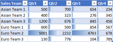
Data bar conditional formatting adds data bars to the cells. By default, the minimum and maximum values in the Range form the bounds and proportional sizes of the data bars. The DataBarConditionalFormat object has several properties to control the bar's appearance.
The following example formats the range with data bars filling left-to-right.
await Excel.run(async (context) => {
    const sheet = context.workbook.worksheets.getItem("Sample");
    const range = sheet.getRange("B8:E13");
    const conditionalFormat = range.conditionalFormats.add(
         Excel.ConditionalFormatType.dataBar
    );

    // Give left-to-right, default-appearance data bars to all the cells.
    conditionalFormat.dataBar.barDirection = Excel.ConditionalDataBarDirection.leftToRight;
    await context.sync();
});
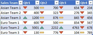
Icon set conditional formatting uses Excel Icons to highlight cells. The criteria property is an array of ConditionalIconCriterion, which define the symbol to be inserted and the condition under which it is inserted. This array is automatically prepopulated with criterion elements with default properties. Individual properties cannot be overwritten. Instead, the whole criteria object must be replaced.
The following example shows a three-triangle icon set applied across the range.
await Excel.run(async (context) => {
    const sheet = context.workbook.worksheets.getItem("Sample");
    const range = sheet.getRange("B8:E13");
    const conditionalFormat = range.conditionalFormats.add(
         Excel.ConditionalFormatType.iconSet
    );

    const iconSetCF = conditionalFormat.iconSet;
    iconSetCF.style = Excel.IconSet.threeTriangles;

    /*
       With a "three*" icon set style, such as "threeTriangles", the third
        element in the criteria array (criteria[2]) defines the "top" icon;
        e.g., a green triangle. The second (criteria[1]) defines the "middle"
        icon, The first (criteria[0]) defines the "low" icon, but it can often
        be left empty as this method does below, because every cell that
       does not match the other two criteria always gets the low icon.
    */
    iconSetCF.criteria = [
        {},
          {
            type: Excel.ConditionalFormatIconRuleType.number,
            operator: Excel.ConditionalIconCriterionOperator.greaterThanOrEqual,
            formula: "=700"
          },
          {
            type: Excel.ConditionalFormatIconRuleType.number,
            operator: Excel.ConditionalIconCriterionOperator.greaterThanOrEqual,
            formula: "=1000"
          }
    ];

    await context.sync();
});
Preset conditional formatting applies a user-defined format to the range based on a selected standard rule. These rules are defined by the ConditionalFormatPresetCriterion in the ConditionalPresetCriteriaRule.
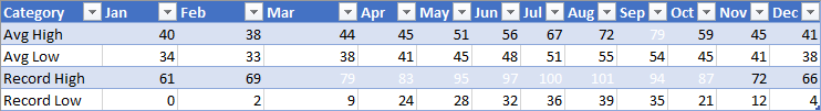
The following example colors the font white wherever a cell's value is at least one standard deviation above the range's average.
await Excel.run(async (context) => {
    const sheet = context.workbook.worksheets.getItem("Sample");
    const range = sheet.getRange("B2:M5");
    const conditionalFormat = range.conditionalFormats.add(
         Excel.ConditionalFormatType.presetCriteria
    );

    // Color every cell's font white that is one standard deviation above average relative to the range.
    conditionalFormat.preset.format.font.color = "white";
    conditionalFormat.preset.rule = {
         criterion: Excel.ConditionalFormatPresetCriterion.oneStdDevAboveAverage
    };

    await context.sync();
});
Text comparison conditional formatting uses string comparisons as the condition. The rule property is a ConditionalTextComparisonRule defining a string to compare with the cell and an operator to specify the type of comparison.
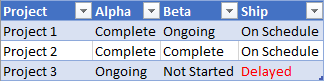
The following example formats the font color red when a cell's text contains "Delayed".
await Excel.run(async (context) => {
    const sheet = context.workbook.worksheets.getItem("Sample");
    const range = sheet.getRange("B16:D18");
    const conditionalFormat = range.conditionalFormats.add(
         Excel.ConditionalFormatType.containsText
    );

    // Color the font of every cell containing "Delayed".
    conditionalFormat.textComparison.format.font.color = "red";
    conditionalFormat.textComparison.rule = {
         operator: Excel.ConditionalTextOperator.contains,
         text: "Delayed"
    };

    await context.sync();
});
Top/bottom conditional formatting applies a format to the highest or lowest values in a range. The rule property, which is of type ConditionalTopBottomRule, sets whether the condition is based on the highest or lowest, as well as whether the evaluation is ranked or percentage-based.
The following example applies a green highlight to the highest value cell in the range.

await Excel.run(async (context) => {
    const sheet = context.workbook.worksheets.getItem("Sample");
    const range = sheet.getRange("B21:E23");
    const conditionalFormat = range.conditionalFormats.add(
         Excel.ConditionalFormatType.topBottom
    );

    // For the highest valued cell in the range, make the background green.
    conditionalFormat.topBottom.format.fill.color = "green"
    conditionalFormat.topBottom.rule = { rank: 1, type: "TopItems"}

    await context.sync();
});
The ConditionalFormat object offers multiple methods to change conditional formatting rules after they've been set.
- changeRuleToCellValue
- changeRuleToColorScale
- changeRuleToContainsText
- changeRuleToCustom
- changeRuleToDataBar
- changeRuleToIconSet
- changeRuleToPresetCriteria
- changeRuleToTopBottom
The following example shows how to use the changeRuleToPresetCriteria method from the preceding list to change an existing conditional format rule to the preset criteria rule type.
Note
The specified range must have an existing conditional format rule to use the change methods. If the specified range has no conditional format rule, the change methods don't apply a new rule.
await Excel.run(async (context) => {
    const sheet = context.workbook.worksheets.getItem("Sample");
    const range = sheet.getRange("B2:M5");

    // Retrieve the first existing `ConditionalFormat` rule on this range.
    // Note: The specified range must have an existing conditional format rule.
    const conditionalFormat = range.conditionalFormats.getItemOrNullObject("0");

    // Change the conditional format rule to preset criteria.
    conditionalFormat.changeRuleToPresetCriteria({
        criterion: Excel.ConditionalFormatPresetCriterion.oneStdDevAboveAverage,
    });
    conditionalFormat.preset.format.font.color = "red";

    await context.sync();
});
You can apply multiple conditional formats to a range. If the formats have conflicting elements, such as differing font colors, only one format applies that particular element. Precedence is defined by the ConditionalFormat.priority property. Priority is a number (equal to the index in the ConditionalFormatCollection) and can be set when creating the format. The lower the priority value, the higher the priority of the format is.
The following example shows a conflicting font color choice between the two formats. Negative numbers will get a bold font, but NOT a red font, because priority goes to the format that gives them a blue font.
await Excel.run(async (context) => {
    const sheet = context.workbook.worksheets.getItem("Sample");
    const temperatureDataRange = sheet.tables.getItem("TemperatureTable").getDataBodyRange();


    // Set low numbers to bold, dark red font and assign priority 1.
    const presetFormat = temperatureDataRange.conditionalFormats
        .add(Excel.ConditionalFormatType.presetCriteria);
    presetFormat.preset.format.font.color = "red";
    presetFormat.preset.format.font.bold = true;
    presetFormat.preset.rule = { criterion: Excel.ConditionalFormatPresetCriterion.oneStdDevBelowAverage };
    presetFormat.priority = 1;

    // Set negative numbers to blue font with green background and set priority 0.
    const cellValueFormat = temperatureDataRange.conditionalFormats
        .add(Excel.ConditionalFormatType.cellValue);
    cellValueFormat.cellValue.format.font.color = "blue";
    cellValueFormat.cellValue.format.fill.color = "lightgreen";
    cellValueFormat.cellValue.rule = { formula1: "=0", operator: "LessThan" };
    cellValueFormat.priority = 0;

    await context.sync();
});
The stopIfTrue property of ConditionalFormat prevents lower priority conditional formats from being applied to the range. When a range matching the conditional format with stopIfTrue === true is applied, no subsequent conditional formats are applied, even if their formatting details are not contradictory.
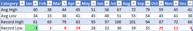
The following example shows two conditional formats being added to a range. Negative numbers will have a blue font with a light green background, regardless of whether the other format condition is true.
await Excel.run(async (context) => {
    const sheet = context.workbook.worksheets.getItem("Sample");
    const temperatureDataRange = sheet.tables.getItem("TemperatureTable").getDataBodyRange();

    // Set low numbers to bold, dark red font and assign priority 1.
    const presetFormat = temperatureDataRange.conditionalFormats
        .add(Excel.ConditionalFormatType.presetCriteria);
    presetFormat.preset.format.font.color = "red";
    presetFormat.preset.format.font.bold = true;
    presetFormat.preset.rule = { criterion: Excel.ConditionalFormatPresetCriterion.oneStdDevBelowAverage };
    presetFormat.priority = 1;

    // Set negative numbers to blue font with green background and
    // set priority 0, but set stopIfTrue to true, so none of the
    // formatting of the conditional format with the higher priority
    // value will apply, not even the bolding of the font.
    const cellValueFormat = temperatureDataRange.conditionalFormats
        .add(Excel.ConditionalFormatType.cellValue);
    cellValueFormat.cellValue.format.font.color = "blue";
    cellValueFormat.cellValue.format.fill.color = "lightgreen";
    cellValueFormat.cellValue.rule = { formula1: "=0", operator: "LessThan" };
    cellValueFormat.priority = 0;
    cellValueFormat.stopIfTrue = true;

    await context.sync();
});
To remove format properties from a specific conditional format rule, use the clearFormat method of the ConditionalRangeFormat object. The clearFormat method creates a formatting rule without format settings.
To remove all the conditional formatting rules from a specific range, or an entire worksheet, use the clearAll method of the ConditionalFormatCollection object.
The following sample shows how to remove all conditional formatting from a worksheet with the clearAll method.
await Excel.run(async (context) => {
    const sheet = context.workbook.worksheets.getItem("Sample");
    const range = sheet.getRange();
    range.conditionalFormats.clearAll();

    await context.sync();
});
Collaborate with us on GitHub
The source for this content can be found on GitHub, where you can also create and review issues and pull requests. For more information, see our contributor guide.
Office Add-ins feedback
Office Add-ins is an open source project. Select a link to provide feedback: